High spatial variability of gas transfer velocity in streams revealed by turbulence measurements

Figures & data

Figure 1. Location of sampling sites and corresponding watershed areas in Sweden.

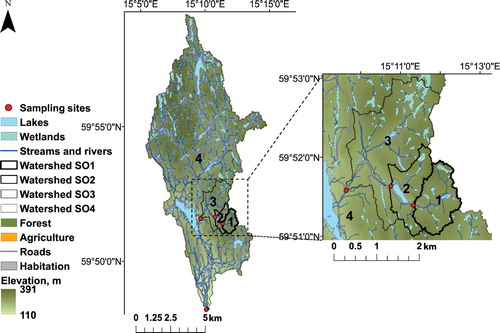
Figure 2. Mean k₆₀₀ for each measurement spot within a reach for (a–b) stream order 1 and 2 in August 2015, (c–d) stream order 1 and 2 in April 2016, and (e–f) stream order 2–4 in June 2016. Data points are based on the 10  min averages used to calculate ε (n = 3–4). Error bars show minimum and maximum values. The x-axes refer to the number of measurement spots.

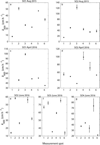
Figure 3. Boxplots of gas transfer velocity (k₆₀₀), pCO₂, pCH₄, and CO₂ and CH₄ emission separated by stream orders (SO) for all sampling occasions; n = number of measurement spots. CO₂ and CH₄ emissions are reported as carbon in g m⁻² d⁻¹. Box shows median value and interquartile range, and whiskers show the adjacent value that is the most extreme data point not considered an outlier. Outliers are illustrated by crosses and are considered above or below 2 standard deviations (2σ) from the mean.

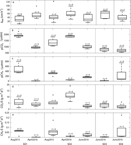
Table 1. Mean horizontal current velocity (U), log-mean of dissipation of turbulent kinetic energy (ε), and gas transfer velocity (k₆₀₀) across stream orders (SO) for all sampling occasions, with min−max in parentheses.

SO	No. meas. spots		No. sampling occasions	Total no. measured spots^a	U (m s^−1)	ε (m^2 s^−3)	k600 (cm h^−1)
1	6		2	11	0.29 (0.019−0.84)	8.6×10^−4 (2.1×10^−6–4.6×10^−2)	42.6 (8.1–99)
2	6		3	17	0.23 (0.015–0.82)	2.8×10^−3 (2.0×10^−6–1.1×10^−1)	50.2 (14.2–123)
3	6		1	6	0.23 (0.05–0.61)	4.2×10^−3 (6.5×10^−4–1.5×10^−2)	57.2 (34.0–75.2)
4	6		1	5	0.45 (0.16–0.73)	1.2×10^−3 (1.1×10^−4–1.6×10^−2)	42.2 (21.7–74.0)

^a The total number of successful measurement spots. Three of the total of 42 measurements were discarded because of uncertain data.

Figure 4. The gas transfer velocity (k₆₀₀) as a function of (a) water current velocity (U) and (b) Reynolds number (Re), both at the logarithmical scale. The color coding reflects the hydraulic diameter (m) of the stream channel for each measurement spot.

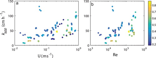
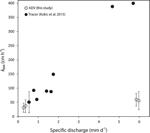
Figure 5. Gas transfer velocity (k₆₀₀) as a function of specific discharge for SO1 and SO2, derived from the eddy cell model (this study; open circles) and tracer injections from Kokic et al. (2015; filled circles). Note that at a k₆₀₀ of ∼50 cm h⁻¹ and a q of ∼0.5 mm d⁻¹, 2 observations overlap, one derived from the tracer-based method and one from the ADV-based method.