Habitat type strongly influences the structural benthic invertebrate community composition in a landscape characterized by ubiquitous, long-term agricultural stress

Figures & data

Figure 1. Sampling points in 3 federal states in Germany.

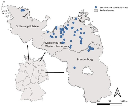
Table 1. Structural composition of communities of waterbodies in arable- and grassland-dominated fields based on 102 samples from arable land and 9 samples from grassland sites. Values in brackets indicate standard deviation. Bold = based on taxonomically harmonized dataset.

	Arable land	Grassland
Species number range	5–89	21–59
Mean number of taxa determined to species	36.8 (16.2)	40.2 (14)
Taxa range after taxonomic harmonization	3–63	21–52
Mean number of taxa	35.3 (12.2)	37.3 (9.6)
EPT-taxa range	0–13	4–14
Mean number of EPT taxa	4.9 (2.8)	10.2 (2.9)
Mean % EPT taxa	20.9 (20.8)	46.3 (24)
Mean % Coleoptera	8.5 (10.2)	3.0 (4.1)
Mean % Odonata	2.6 (3.4)	4.6 (4.5)
Mean % Chironomidae	21 (21.7)	10.9 (14.8)
Shannon index, mean values	1.9 (0.6)	2.1 (0.4)
Evenness index, mean values	0.5 (0.1)	0.6 (0.1)

Table 2. Overview of environmental parameters and day of sampling based on 102 samples from arable land and 9 samples from grassland sites. Values in brackets indicate standard deviation.

	Arable land	Grassland
Mean number of habitats (1–4)	1.6 (0.7)	1.3 (0.5)
Mean toxicity (TUmax)	−3.6 (1.7)	−3.7 (1.3)
Mean ammonium (NH4^+) [mg N/L]	0.3 (0.7)	0.1 (0.2)
Mean nitrate (NO3^−) [mg N/L]	5.5 (12.1)	0.1 (0.0)
Mean phosphate (PO4^3−) [mg P/L]	0.6 (1.1)	0.1 (0.1)
Mean pH	8.0 (0.7)	8.1 (0.4)
Mean temperature [°C]	14.0 (4.6)	10.1 (1.9)
Mean oxygen content [mg/L]	10.5 (2.7)	10.5 (3.2)
Mean EC (electronic conductivity) [µS/cm]	582.8 (456.0)	394.1 (191.3)
DOY (day of the year of sampling)	115.3 (15.4)	110.4 (12.3)

Table 3. Results for the model-averaged coefficients (full average) of the GLMs. Significant p values are given for the variables. Significant interaction terms are listed in the last column with their respective p value. For all response variables a Gaussian family link was used. n = number of samples in the dataset, DOY is day of year, T is temperature, EC is electrical conductivity.

	No. of habitats	Habitat type	Land use	DOY	Toxicity	NH4^+	NO3^−	PO4^3−	pH	T	O2	EC	Interaction terms
Shannon-index (n = 105)	0.0625 (hab_2)	NA	—	—	—	—	—	—	—	—	—	—	—
Single-habitat (n = 59)	NA	—	—	0.00759	—	0.03882	—	0.02223	—	0.04365	—	—	0.00222 (NH4^+:NO3^−) 0.00266 (NH4^+:PO4^3-) 0.01178 (NH4^+:toxicity) 0.00604 (NO3^−:toxicity) 0.00518 (NH4^+:NO3^−:PO4^3−)
Multi-habitat (n = 46)	NA	NA	—	—	—	—	—	—	—	—	—	—	—
arable-single-habitat types (3) (n = 51)	NA	2.01x10^-5 (macrophytes) 9.60x10^-6 (reed)	NA	0.01936	—	—	—	0.00690	—	0.03761	—	0.03299	0.03399 (NO3^−:toxicity) 0.02188 (PO4^3−:toxicity) 0.00632 (NH4^+:NO3^−:PO4^3-)
Single-habitat types (3) (n = 56)	NA	0.000116 (macrophytes); 5.3x10^-6 (reed)	—	—	—	0.025529	—	—	—	0.045633	—	—	0.002740 (NH4^+:NO3^−) 0.015535 (NH4^+:PO4^3−) 0.018133 (NH4^+:toxicity)
Evenness-index (n = 105)	—	NA	—	—	—	—	—	—	0.03815	—	—	0.00493	0.00705 (NH4^+:NO3^−:toxicity)
EPT taxa (n = 105)	—	NA	4x10^-7	0.02579	0.00255	—	—	—	—	0.0022	—	—	—
arable (n = 97)	—	NA	NA	—	0.00474	—	—	—	—	0.00399	—	—	—
Taxa number (n = 105)	5.2x10^-6 (hab_2) 0.002110 (hab_3) 6.9x10^-6 (hab_4)	NA		0.000152	—	—	—	—	—	—	—	—	—
Arable land (n = 97)	2.4x10^-6 (hab_2) 0.000929 (hab_3) 8.5x10^-6 (hab_4)	NA	NA	0.000308	—	—	—	—	—	—	—	—	—
Single-habitat arable (n = 54)	NA	—	NA	0.00471	—	—	—	—	—	—	—	—	—
Multi-habitat arable (n = 43)	NA	NA	NA	2.12x10^-5	—	—	—	—	—	—	—	—	—
Single-habitat (n = 59)	NA	—	—	0.00095	—	—	—	—	—	—	—	—	—
Single-habitat types reduced (n = 56)	NA	0.00216 (macrophytes); 4.4x10^-6 (reed)	—	0.00182	—	—	—	—	—	—	—	—	—
Multi-habitat (n = 46)	NA	NA	—	3.45x10^-5	—	—	—	—	—	—	—	—	—

Table 4. Results of the PERMANOVA run separately for the grouping variables. The values give the difference between the groups in percent. Values in brackets are the p values. n = number of samples in the dataset. Five habitat types^† (CPOM, FPOM, reed, macrophytes, and others; 3 habitat types^‡ (CPOM/FPOM, reed, macrophytes).

	Habitat (single/ multi)	Land use (arable/ grassland)	Sampling (early/late)	Toxicity (polluted/ less polluted)	Habitat type (5^† or 3^‡)
Hellinger-transformed community data (n = 105)	1.6 (0.051)	3.0 (0.001)	3.5 (0.001)	1.5 (0.0049)	NA
Single-habitat (n = 59)^†	NA	3.4 (0.008)	4.0 (0.005)	2.6 (0.078)	13.7 (0.001)
Arable, single-habitat (n = 54)^†	NA	NA	4.6 (0.002)	3.0 (0.055)	15.7 (0.001)
Arable, single-habitat (n = 51)‡	NA	NA	5.0 (0.006)	3.0 (0.068)	10.5 (0.001)
Multi-habitat (n = 46)	NA	5.6 (0.001)	4.5 (0.003)	3.7 (0.028)	NA
Presence-absence transformed community data (n = 105)	1.9 (0.008)	4.1 (0.001)	3.9 (0.001)	1.9 (0.018)	NA
Single-habitat (n = 59)^†	NA	5.1 (0.001)	4.1 (0.002)	2.8 (0.052)	13.7 (0.002)
Arable, single-habitat (n = 54)^†	NA	NA	5.0 (0.001)	3.1 (0.046)	15.9 (0.001)
Arable, single-habitat (n = 51)^‡	NA	NA	5.4 (0.001)	4.3 (0.007)	8.9 (0.001)
Multi-habitat (n = 46)	NA	5.3 (0.007)	5.9 (0.001)	3.4 (0.073)	NA

Table 5. Contributions of species to differences between groups. For each dataset and variable, the first 5 species are shown with their respective contribution (averages) to the group differences. Values are given in percent. Calculated using the simper function, vegan package in R (Oksanen et al., 2022). Community data for this analysis was presence–absence transformed.

	Full dataset (n = 105)				Arable, single-habitat samples, habitat type (n = 51)
	Habitat (single/ multi)	Land use (arable/ grassland)	Sampling (early/late)	Toxicity (polluted/less polluted)	Reed vs. macro-phytes	Reed vs. CPOM/FPOM	Macro-phytes vs. CPOM/FPOM
Caenis horaria		1.206
Athripsodes aterrimus		1.103
Hippeutis sp.		0.955
Triaenodes bicolor		0.95
Oectis furva		0.884
Hygrotus sp.	0.799		0.755
Hydroporus sp.	0.779
Cataclysta sp.	0.741
Dytiscinae Gen. sp.	0.729		0.786	0.748
Agabus sp.	0.729
Asellidae Gen. sp.			0.77	0.789		1.22
Limnephilus flavicornis			0.801			1.264
Hydrobius sp.			0.839	0.784
Corduliidae/Libelluidae Gen. sp.	0.733			0.768
Segmentina sp.				0.745	0.919
Culicidae Gen. sp.						1.33	1.351
Scirtidae Gen. sp.						1199
Limoniidae Gen. sp.						1.203
Limnephilus vittatus					0.947		1.364
Helochares sp.					0.95
Anacaena sp.					0.939
Stratiomyidae Gen. sp.							1.397
Enochrus sp.					0.97		1.621
Colymbetinae Gen. sp.							1.241

Table 6. Results from the pRDA. Latitude and Longitude used as input for the conditioned variance. Variable outcome from the backward selection of the RDA plus toxicity and number of habitats. Hellinger-transformed dataset used. n = number of samples in the dataset.

	Significant variables after backward selection + toxicity + habitat number	Conditioned variance explained in %	Constrained variance explained in %	Adjusted R^2 of constrained variance explained in %
Complete dataset (n = 105)	PO4^3− + EC + pH + land use + DOY + toxicity + habitat number	3.1	15.8	8.1
single-habitat SWBs (n = 59)	EC + pH + DOY + habitat type + toxicity	3.5	23.3	11.5
single-habitat SWBs reduced (grouped to three habitats (n = 56)	EC + pH + DOY + habitat type + toxicity	9.1	21.3	12.9
multi-habitat SWBs (n = 46)	NO3^− + DOY + toxicity + habitat number	5.8	18.1	6.0
Arable land (n = 97)	EC + pH + DOY + toxicity + habitat number	3.5	12.4	5.8
single-habitat SWBs (n  =54)	EC + pH + DOY+ habitat type + toxicity	4.0	25.1	12.4
single-habitat SWBs (n = 51 with grouped [3 groups] habitat type as parameter)	EC + pH + DOY+ habitat type + toxicity	4.3	23.1	13.2
multi-habitat SWBs (n = 43)	NO3^− + DOY + toxicity + habitat number	6.3	13.7	2.5

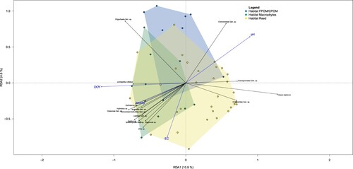
Figure 2. Ordination diagram of first 2-axis pRDA analysis based on the Hellinger-transformed abundance data, conditioned for spatial variation. Environmental parameters with continuous values (DOY, toxicity, EC, pH) are shown as blue arrows. Environmental parameter habitat described as a factor is shown as colored polygons. Species that explain at least 25% of variation are shown as black arrows. Gen. sp. denotes grouping that includes genera/species

Data availability statement

Due to the sensitive nature of the questions asked in this study, farmers were assured raw data would remain confidential and would not be shared, and respondents would not be identified individually. All data on the analytical methods can be requested from the authors.