Determination of optimal potential parameters for the self-assembly of various lattice structures

Figures & data

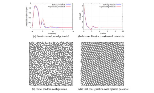
Figure 1. Smoothed Gaussian potential in reciprocal space; depending on the magnitude of smoothing parameter $\sigma ,$ appropriately regular Gaussian potential can be generated.

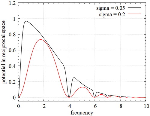
Figure 2. Designed potentials for various lattices-Fourier transformed potential (left), and Inverse Fourier-transformed potential (right); The potential in the original space increases drastically as reducing the radius. However, in reciprocal space, the shape of potential is more controllable.

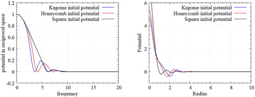
Figure 3. Particle configurations by ansatz potentials for target Kagome(left), honeycomb(center), and square(right) lattices in annealing simulations. Such ansatz potentials form the Bravais lattices of the target structures directly. Since a gradient based optimization converges to a local minimum, an adequate choice of ansatz potentials is essential.

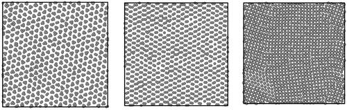
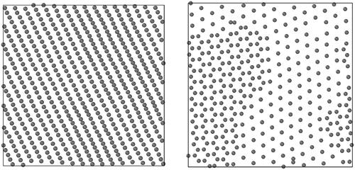
Figure 4. Particle configurations for the self-assembly of honeycomb lattice at the initial time step (left) and the final time step with the optimal potential (right); With the obtained optimal potential, the particles are randomly distributed at initial simulation, and then are cooled down steadily until sufficient crystallization occurs.

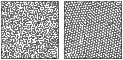
Figure 5. Comparison of RDFs for honeycomb lattice with target(black), initial(blue) and optimal(red) potentials; The obtained RDF of optimal potential is almost the same as that of the target lattice. The peak height of the first coordinate shell differs significantly from that of the target lattice, which is caused from the several defects but the heights of peak can be changed with temperature conditions.

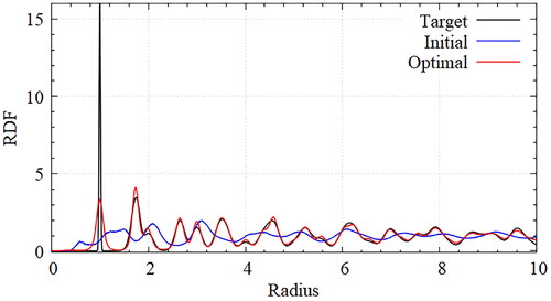
Figure 6. Designed potential for honeycomb Lattice – Fourier transformed potential(left) and inverse Fourier transformed potentials(right); The frequency range of 5–10 is highly sensitive for the optimal design of potential due to its significant influence on the fluctuation of potential in the real space.

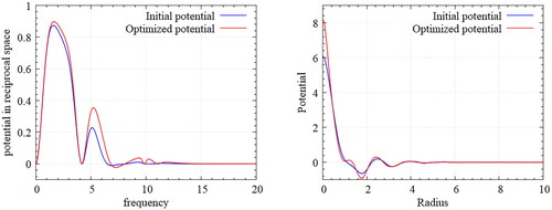
Figure 7. Optimization history for honeycomb structure; The history of difference between the target and the designed RDFs in Eq. (22)(22) $$\sum _i\left[\frac{d{\alpha }_i}{d{p}_l}{\widehat{V}}_i({\sigma }_i,G_i;G_l)+{\alpha }_i\frac{d{\widehat{V}}_i({\sigma }_i,G_i;G_l)}{d{p}_l}\right]=0.$$(22) is plotted as we perform the simulations. Some fluctuations are observed but eventually the RDF by the optimal design is markedly decreased.

Figure 8. Particle configurations in Kagome lattice – Final configuration with optimal potential (left), Configuration net for visualization (right); The configuration net shows the connectivity of adjacent particles for the easy visualization of lattice structure.

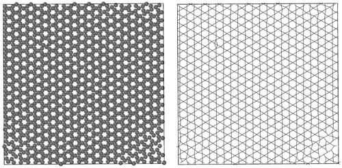
Figure 9. Comparison of RDFs for Kagome lattice; Compared to the target lattice, the peak of coordinate shell is slightly different. However, its position is almost identical and the difference can be reduced by controlling the temperature of simulations.

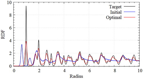
Figure 10. Designed potential for Kagome Lattice – Fourier transformed potential (left), Inverse Fourier transformed potentials (right).

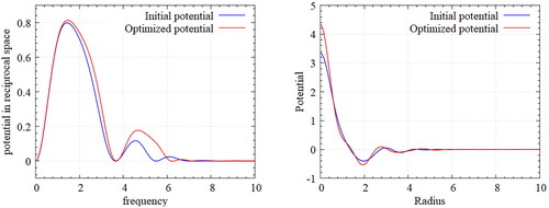
Figure 11. Optimization history for Kagome structure; Some fluctuations of the fitness measure in Eq. (26)(26) $${\varphi }^2=\int {\left(g_{*}(r)-g_T(r)\right)}^{2}dr,$$(26) are observed but the overall tendency is decreasing.

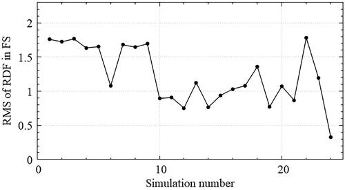
Figure 12. Energy per atom with designed potentials for the honeycomb lattice (dotted) and the Kagome lattice (solid) according to density variations; Each potential was designed at a specified density (red circles).

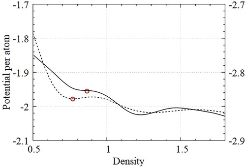
Figure 13. Self-assembled configuration with a designed potential at low density condition – Kagome lattice (left, density 0.66), honeycomb lattice (bottom, density 0.54); In case the density deviates to a certain extent, a stripe pattern can be obtained for Kagome lattice (left) and a triangular lattice with twice unit length for honeycomb lattice (right).

Data availability

The data that support the findings of this study are available from the corresponding author upon reasonable request.