Figures & data
Figure 1. Images showing some of the defected engineering structures in the study area. The red arrows indicate reinforcements (concrete patching and buttress supports), while the red circles show the sections of the highway with pavement defects
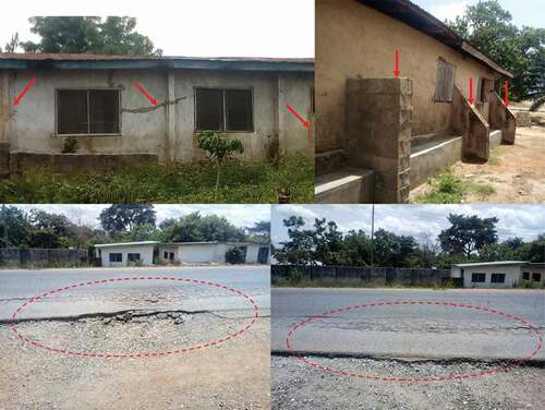
Figure 2. (a) Regional geological map of Nigeria within the Pan-African mobile belt between the West African and Congo Cratons. (b) Outline geological map of Nigeria showing Etioro-Akoko in the southwestern Nigerian Basement Complex (modified after Woakes et al. Citation1987)
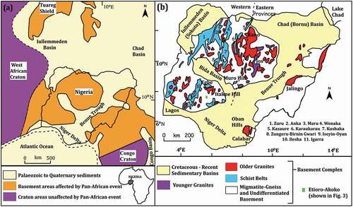
Figure 3. Geological map of Etioro-Akoko and its environs, Ondo State, southwestern Nigeria
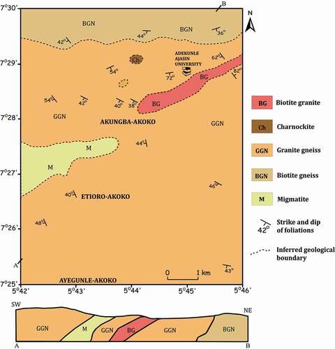
Figure 4. (a) Data acquisition map of the study area showing all the geophysical traverses and existing boreholes and wells. (b) 3-dimensional (3D) electrode array diagram showing the surface relief of the study area, geophysical traverses, and the positions of the electrodes along each traverse. Inset: location map of Ondo state showing the study area
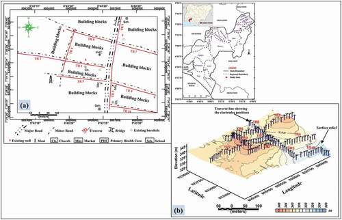
Figure 5. The inverse model resistivity sections of TRs 1–10 (a–j). The slanting broken lines (F – F’) indicate the bedrock fractures.
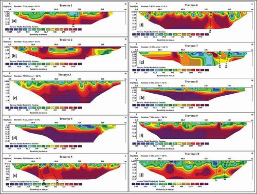
Figure 6. 2D inverted resistivity depth slice map of the study area at depth: (a) 0 – <1 m (top layer), (b) 5 m, (c) 10 m, (d) 15 m, (e) 20 m and (f) 25 m. The maps depict the spatial distribution of the subsurface resistivities at various depths. The traverse lines were superimposed on map “A” to show the constraint of data sets to their exact position.
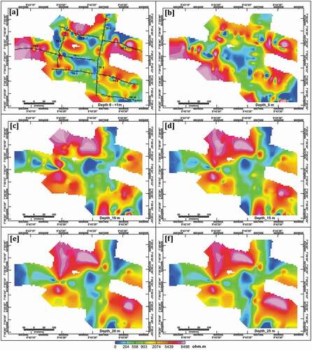
Figure 7. 2D contoured bedrock surface map of the study area (top panel) showing the litho-section lines with their resulting litho-section profiles (down panels) along NE-SW (a), NW-SE (b), NS (c) and E-W (d). The litho-sections show the depths to fresh bedrock, undulating bedrock topography, and weak zones in the area. A negative depth value implies depth below ground level (bgl).
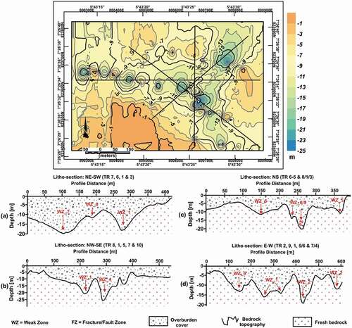
Figure 8. Bedrock structural map of the study area showing the variations in overburden thicknesses and trends of the subsurface fractures (F 1–5)
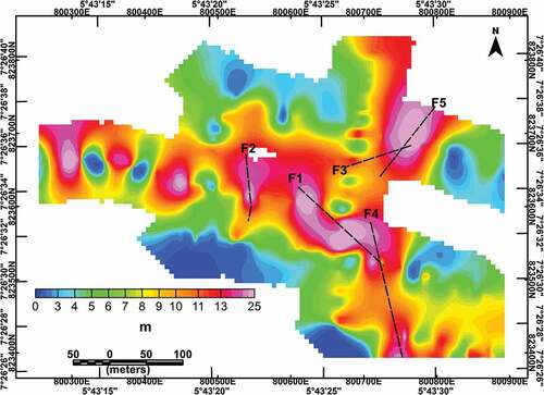
Figure 9. 3D geotomographic depths slice model showing the depth limits for the delineated fractures (in broken circles and annotated as A, B and C). The negative depth values imply depth bgl
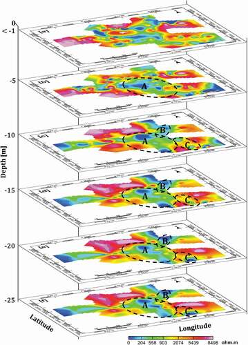
Figure 10. Idealised composite image of the subsurface inverted resistivity models of the study area. It shows the litho-structural dynamics, proposed hand-dug well and borehole points, and proposed bridges for failed road sections.
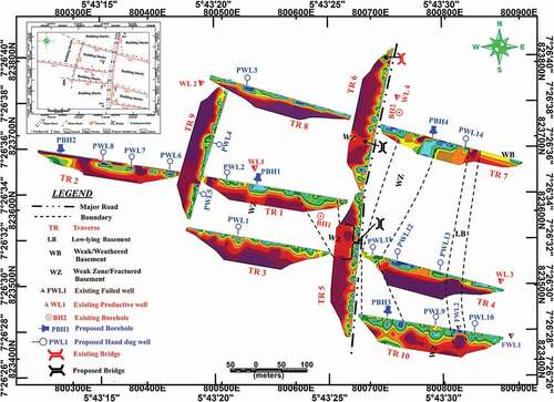
Table 1. A comprehensive summary of the locations, approximate drill depths, widths and the nature and geological conditions of aquifers proposed for siting of hand-dug wells and boreholes in the study area
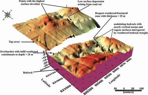
Figure 11. 3D conceptualised soil-lithology thickness model of the study area showing the variability patterns of the topographic relief, weathering thickness and bedrock structural architecture