A reconnaissance study for tracing and ordering new mineralisation zones using integrated remote sensing, GIS, and aeromagnetic techniques, west Allaqi-Heiani-Suture,Egypt

Figures & data

Figure 1. (a) Location of the study area. (b) A simplified geological map of the Egyptian Eastern Desert highlights the general geology and position of the study area (modified after Ramadan et al. 2001; Abdelsalam et al. 2003; Abdelsalam 2010; Johnson et al. 2011, 2017; Azer 2013; ElGalladi et al. 2022). (c) Detailed geological map of west Allaqi-Heiani Suture (AHS) (Kusky and Ramadan 2002; ElGalladi et al. 2022).

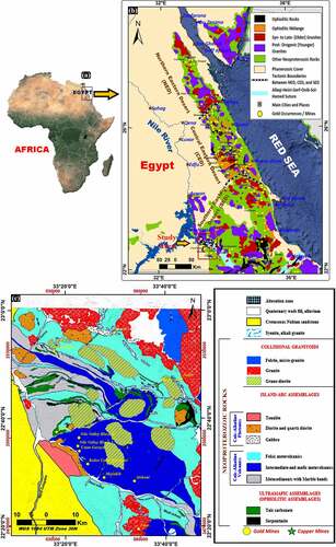
Figure 2. (a) Drainage system over west Allaqi district. (b) 3D view simulates the topography setting with the drainage network.

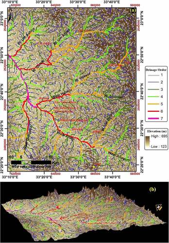
Figure 3. A flowchart scheme shows the processing techniques used for the exploration of new prospective mineralisation potential zones over the west Allaqi-Heiani Suture (AHS).

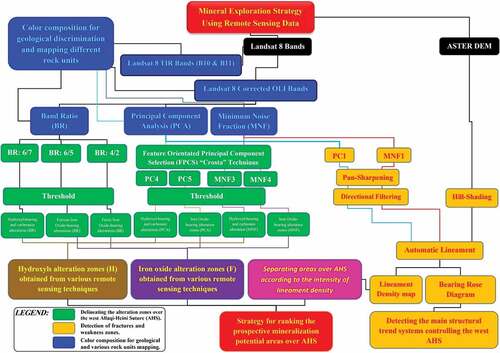
Table 1. Statistical factors used for estimating the band ratios threshold values for mapping alteration minerals in Figure 4.

Alteration Minerals	Ratio	Min.	Max.	Mean	Standard Deviation	Threshold	Confidence %
Hydroxyls & Carbonates	BR 6/7	0	255	112.21	59.9	232.01	95%
Ferrous-Irons	BR 6/5	0	255	75.47	53.24	235.2	98%
Ferric-Irons	BR 4/2	0	255	96.55	70.65	237.85	95%

Figure 4. Threshold of band ratios 6/7, 6/5 and 4/2 to extract alteration zones: (a) Hydroxyl-bearing and carbonate minerals extraction, BR 6/7. (b) Extraction of ferrous-iron oxide minerals, BR 6/5. (c) Extraction of ferric-iron oxides minerals, BR 4/2. (d) The alteration minerals overlaid the natural colour image of Google Earth.

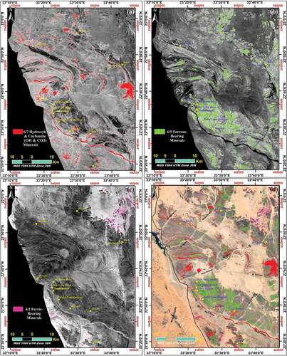
Table 2. PCA eigenvector matrix of Landsat 8 used bands (B1–B7).

Landsat 8	Band 1	Band 2	Band 3	Band 4	Band 5	Band 6	Band 7	Variances in PCn (%)
PC 1	−0.0824	−0.1069	−0.2289	−0.4016	−0.4695	−0.55	−0.4952	95.8
PC 2	0.4632	0.498	0.5021	0.2524	0.0732	−0.3781	−0.2708	3.36
PC 3	−0.3814	−0.341	−0.0337	0.473	0.4997	−0.2144	−0.4666	0.61
PC 4	−0.1287	−0.0799	−0.0091	0.0289	0.1428	−0.7097	0.6724	0.19
PC 5	−0.1243	−0.1591	0.1218	0.6578	−0.7068	0.0252	0.1074	0.05
PC 6	−0.4358	−0.1833	0.8088	−0.3395	−0.0567	0.0623	−0.0018	0
PC 7	0.6394	−0.7484	0.1628	−0.0515	0.0368	−0.02	0.009	0

Figure 5. (a) Extraction of hydroxyl-bearing and carbonate minerals by thresholding the inverted PC4. (b) Extraction of iron oxide minerals by thresholding the inverted PC5. (c) Extraction of hydroxides and iron oxides by thresholding the inverted (PC4+ PC5). (d) Crosta’s FCC image of inverted PC4, inverted (PC4+ PC5) and inverted PC5 as RGB.

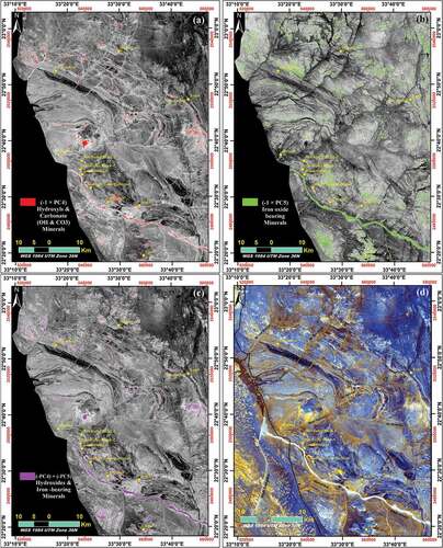
Figure 6. (a) Extraction of hydroxyl-bearing and carbonate minerals by thresholding MNF3. (b) Extraction of iron oxide minerals by thresholding MNF4. (c) Extraction of hydroxides and iron oxide minerals by thresholding MNF3 + MNF4 image. (d) Crosta alteration image, FCC image of MNF3, (MNF3+ MNF4) and MNF4 respectively as RGB.

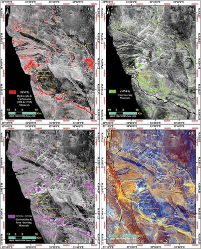
Table 3. Eigenvectors of MNF components of Landsat 8 used bands (B1-B7).

Landsat 8	Band 1	Band 2	Band 3	Band 4	Band 5	Band 6	Band 7
MNF1	−0.3594	0.4405	0.7147	0.0006	0.3957	−0.0079	0.097
MNF2	0.8742	0.0444	0.3129	−0.2123	0.1724	−0.2471	0.0103
MNF3	0.2962	0.4777	0.0485	0.6225	−0.3312	0.427	−0.0479
MNF4	−0.0292	−0.6265	0.4381	0.5081	−0.0332	−0.1365	−0.3699
MNF5	0.133	−0.3098	−0.1413	0.1818	0.649	0.5465	0.3367
MNF6	−0.0079	−0.2864	0.3747	−0.1769	−0.5214	0.2105	0.6557
MNF7	0.0187	−0.0723	0.1915	−0.4949	−0.0992	0.6284	−0.555

Figure 7. (a) Remotely sensed combination of lineaments extracted automatically from the composition of enhanced PC1, MNF1 and DEM images. (b) Remote sensed lineament density map of west AHS. (c) Lineaments orientation rose diagram. (d) Lineaments length rose diagram. (e) Basic statistics of the total automatically extracted lineaments.

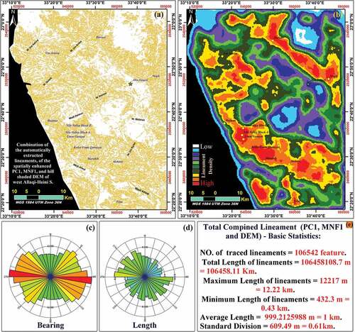
Figure 8. Automatically, remotely sensing, extracted lineaments for alteration zones: (a) Lineaments of hydroxyl-bearing zones. (b) Lineaments of iron-oxide altered zones. (c) Lineaments orientation rose diagram of hydroxyl-bearing zones. (d) Lineaments length rose of hydroxyl altered zones. (e) Lineaments trend rose diagram of iron-oxides. (f) Lineaments length rose diagram of iron-oxide altered zones.

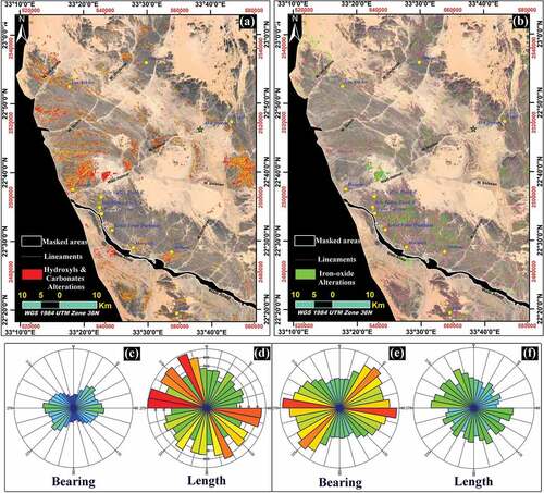
Figure 9. (a) RTP map. (b) Tilt derivative (TDR) map. (c) Zero contours of TDR map to outline the edges of magnetic anomalies, with their rose diagram. (d) Euler solutions estimated the depths to magnetic contacts at shallow depths (≤−150 m), with their rose diagram (ElGalladi et al. 2022).

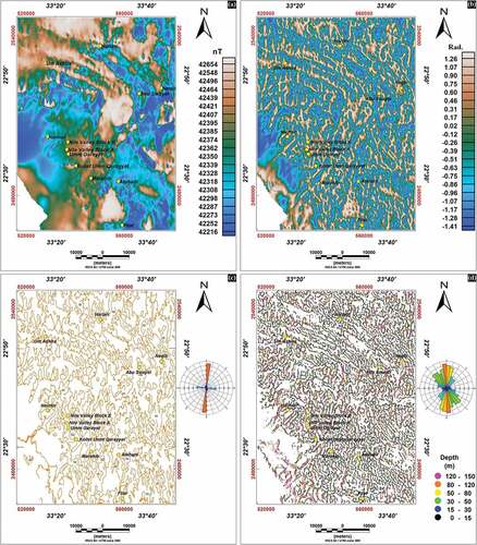
Figure 10. (a) Analytic signal map of the total magnetic field (AS). (b) Analytic signal of the first vertical derivative (AS1). (c) Depth estimations to the magnetic sources using the analytic signal technique. (d) Depth solutions to the magnetic sources/contacts, beneath AHS, using the SPI technique.

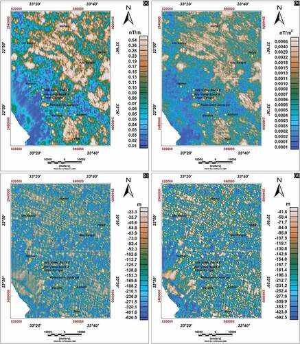
Figure 11. (a) 3D gridding, (b) 3D symbol simulation, of the depths to magnetic sources/contacts estimated using the SPI technique which suggests a ductile–brittle transitional/deformational zone (DBZ).

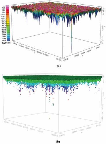
Figure 12. Landsat 8 band composition images over the west AHS. (a) Pan-sharpened natural (true) colour of OLI band composition as Red: B4, Green: B3 and Blue: B2. (b): (g) False colour composite (FCC) images using OLI and TIRS bands, band ratios and PCA images. (Bands included in the FCC composition, in the RGB channels, are labelled over each image).

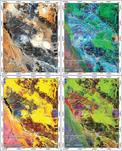
Figure 12. (Continued).

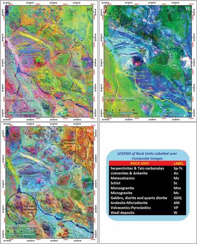
Table 4. Geological maps that were used for correlation and labelling the Landsat 8, TCC and FCC, images over the west Allaqi-Heiani Suture (AHS).

Geological Map	Reference
West Allaqi-Heiani Suture area	CONOCO (1987); EGSMA (1996); Kusky and Ramadan (2002); Abdelsalam et al. (2003); Zoheir et al. (2018); Eldosouky et al. (2017).
Wadi Shalman area (east central study area)	Abdeen and Abdelghaffar (2008); Azer (2013).
Wadi Haimur area (west central study area)	Khalil et al. (2014).
Haimur gold mine area	Emam and Zoheir (2013); Zoheir and Emam (2014); Ramazanov and Ali (2012).
Um Garayat (Umm Qurayyat) gold mine area	El-Makky and Sediek (2012); Zoheir et al. (2018).
Marahib (Marahiq) gold mine area	Emam et al. (2014).
Um Ashira gold mine area	El-Desoky et al. (2021); Emam and Radwan (2021).

Figure 13. (a) Superimposing image combines hydroxyl-bearing, iron-oxide alterations and fracture system, the highest earlier three lineament density contours, all over a real colour image of Google Earth. (b) Remotely sensed ranking of the prospective mineralisation zones in west AHS, Diagram, c represents a legend of the probable mineralisation categories. (c) The pyramid scheme describes the ranking order of prospective mineralisations according to the existence of alteration zones and the structural control system. The top of the diagram (red colour) represents the highest ranking (first order) of the probable mineralisation occurrences, while the bottom is the expected lowest potential ranking.

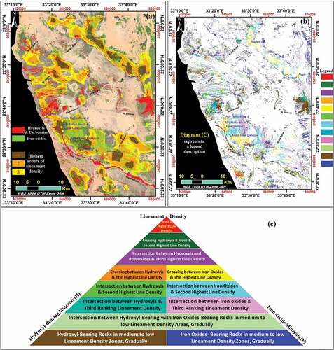
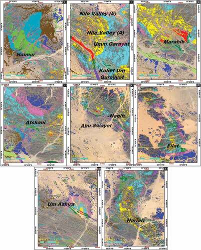
Figure 14. Comparison between the remotely sensed ordering with the known gold mines in west AHS, overlie Google Earth images: (a) Haimur gold mine. (b) Nile Valley Blocks and Um Garayat gold mines. (c) Marahib gold mine. (d) Atshani gold mine. (e) Nagib gold mine and area of Abu Swayel copper mine. (f) Filat gold mine. (g) Um Ashira gold mine. (h) Hariari gold mine. Diagram, c, in Figure 13, represents a legend of the colours in this figure (Figure 14) and describes the ranking order of the prospective mineralisation occurrences.

Ramadan T, Abdelsalam M, Stern R. 2001. Mapping gold-bearing massive sulfide deposits in the Neoproterozoic Allaqi Suture, Southeast Egypt with Landsat TM and SIR=C/X SAR Images. Photogramm Eng Remote Sensing. 67(4):491–497.

 Web of Science ®Google Scholar

Abdelsalam MG, Abdeen MM, Dwaidar HM, Stern RJ, Abdelghaffar AA. 2003. Structural evolution of the Neoproterozoic western Allaqi-Heiani Suture, southeastern Egypt. Precambrian Res. 124(1):87–104. doi:10.1016/S0301-9268(03)00080-9.

 Web of Science ®Google Scholar

Abdelsalam MG. 2010. Quantifying 3D post-accretionary tectonic strain in the Arabian–Nubian Shield: superimposition of the Oko Shear Zone on the Nakasib Suture, Red Sea Hills, Sudan. J Afr Earth Sci. 56(4–5):167–178. doi:10.1016/j.jafrearsci.2009.07.003.

 Web of Science ®Google Scholar

Johnson P, Andresen A, Collins A, Fowler A, Fritz H, Ghebreab W, Kusky T, Stern R. 2011. Late Cryogenian–Ediacaran history of the Arabian–Nubian Shield: a review of depositional, plutonic, structural, and tectonic events in the closing stages of the Northern East African Orogen. J Afr Earth Sci. 61(3):167–232. doi:10.1016/j.jafrearsci.2011.07.003.

 Web of Science ®Google Scholar

Johnson P, Zoheir B, Ghebreab W, Stern R, Barrie C, Hamer R. 2017. Gold-bearing volcanogenic massive sulfides and orogenic-gold deposits in the Nubian Shield. South Afr J Geol. 120(1):63–76. doi:10.25131/gssajg.120.1.63.

 Web of Science ®Google Scholar

Azer MK. 2013. Evolution and economic significance of listwaenites associated with Neoproterozoic ophiolites in south Eastern Desert, Egypt. Geologica Acta. 11(1):113–128.

 Web of Science ®Google Scholar

ElGalladi A, Araffa S, Mekkawi M, Abd-AlHai M. 2022. Exploring mineralization zones using remote sensing and aeromagnetic data, West Allaqi area, Eastern-Desert, Egypt. Egypt J Remote Sens Space Sci. 25(2):417–433. doi:10.1016/j.ejrs.2022.03.007.

 Web of Science ®Google Scholar

Kusky T, Ramadan T. 2002. Structural controls on Neoproterozoic mineralization in the South Eastern Desert, Egypt: an integrated field, Landsat TM, and SIR-C/X SAR approach. J Afr Earth Sci. 35(1):107–121. doi:10.1016/S0899-5362(02)00029-5.

 Web of Science ®Google Scholar

CONOCO. 1987. Geological map of Egypt, Bernice Sheet, NF 36 NE, Scale 1: 500,000. The Egyptian general petroleum corporation (EGPC). Cairo (Egypt).

 Google Scholar

EGSMA. 1996. Geological map of Wadi Jabjabah Quadrangle, Egypt, NF-36-K. scale. 1: 250:000.

 Google Scholar

Zoheir B, Emam A, Pitcairn I, Boskabadi A, Lehaye Y, Cooper M. 2018. Trace elements and isotope data of the Um Garayat gold deposit, Wadi Allaqi district, Egypt. Miner Depos. 54(1):101–116. doi:10.1007/s00126-018-0807-3.

 Web of Science ®Google Scholar

Eldosouky A, Abdelkareem M, Elkhateeb S. 2017. Integration of remote sensing and aeromagnetic data for mapping structural features and hydrothermal alteration zones in Wadi Allaqi area, South Eastern Desert of Egypt. J Afr Earth Sci. 130:28–37. doi:10.1016/j.jafrearsci.2017.03.006

 Web of Science ®Google Scholar

Abdeen MM, Abdelghaffar AA. 2008. Mapping Neoproterozoic structures along the central Allaqi-Heiani suture, southeastern Egypt, using remote sensing and field data. Egypt J Remote Sens Space Sci. 11:109–138.

 Google Scholar

Khalil A, Obeid M, Azer M. 2014. Serpentinized Peridotites at the North Part of the Wadi Allaqi district (Egypt): implications for the tectono-magmatic evolution of fore-arc crust. Acta Geol Sin (Engl Ed). 88(5):1421–1436. doi:10.1111/1755-6724.12309.

 Web of Science ®Google Scholar

Emam A, Zoheir B. 2013. Au and Cr mobilization through metasomatism: microchemical evidence from ore-bearing listvenite, South Eastern Desert of Egypt. J Geochem Explor. 125:34–45. doi:10.1016/j.gexplo.2012.11.004

 Web of Science ®Google Scholar

Zoheir B, Emam A. 2014. Field and ASTER imagery data for the setting of gold mineralization in Western Allaqi–Heiani belt, Egypt: a case study from the Haimur deposit. J Afr Earth Sci. 99(1):150–164. doi:10.1016/j.jafrearsci.2013.06.006.

 Google Scholar

Ramazanov V, Ali M. 2012. Prediction of gold potential areas based on remote sensing techniques: a case study from Wadi Haimur region, South–Eastern Desert, Egypt. Baki Universitetinin X?b?rl?ri, T?bi?t Elml?ri Seriyasi ?1. 55(6):99–109.

 Google Scholar

El-Makky A, Sediek N. 2012. Stream sediments geochemical exploration in the northwestern part of Wadi Allaqi area, south Eastern Desert, Egypt. Nat Resour Res. 21(1):95–115. doi:10.1007/s11053-011-9166-9.

 Google Scholar

Emam A, Qaoud N, Abdel Rahman E, Fawzy K. 2014. Comprehensive mapping of the island arc rocks in the Marahiq area, South Eastern Desert, Egypt. Open Geology J. 8(1):84–96. doi:10.2174/1874262901408010084.

 Google Scholar

El-Desoky H, Soliman N, Heikal M, Abdel-Rahman A. 2021. Mapping hydrothermal alteration zones using ASTER images in the Arabian–Nubian Shield: a case study of the northwestern Allaqi District, South Eastern Desert, Egypt. Asian Earth Sci: X. 5:100060. doi:10.1016/j.jaesx.2021.100060

 Web of Science ®Google Scholar

Emam A, Radwan A. 2021. Geochemistry and petrogenesis of I-type granitoid rocks around Nasb-Zurar intrusion, West Wadi Allaqi, South Eastern Desert, Egypt. Arab J Geosci. 14(7). doi:10.1007/s12517-021-06913-x.

 Google Scholar

Data availability statement

The data collected for this work are available.