Shallow subsurface investigations for soil properties at Pedas, Negri Sembilan, Peninsula Malaysia using MASW, ERT,IP, and TEM methods

Figures & data

Figure 1. Simplified geology of Negeri Sembilan (After Arisona et al. 2017) and the layout of the site (lower right).

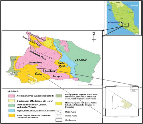
Figure 2. Location map of geophysical field layout adopted in the present work.

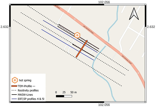
Table 1. Resistivity values of some subsurface rocks and soil materials (after Keller George and Frischknecht Frank 1996).

Material	Resistivity (Ω-m)
Alluvium	10 to 100
Sand	60 to1000
Clay	1 to 100
Groundwater (fresh)	10 to 100
Granite	5000 to 1,000,000

Table 2. Earth materials and chargeability properties (modified after Murali and Patangay (2006).

Earth material	Chargeability (ms)
Water	0
Alluvium	1–4
Gravel	3–9
Sandstone	3–12
Quartzite	5–12
Schist	5–20
Argillites	5–10
Precambrian gneisses	6–30

Figure 3. Shear wave velocity inversion of line 1 in the study area.

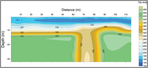
Figure 4. Shear wave velocity model of line 2 in the study area.

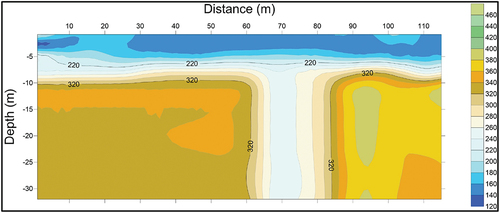
Figure 5. Shear wave velocity model of line 3 in the study area.

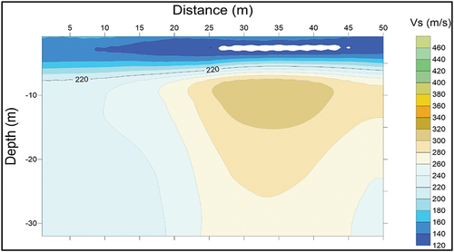
Figure 6. Shear wave velocity depth slice at 5m in the study area.

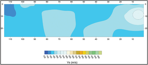
Figure 7. Shear wave velocity depth slice at 18.5m in the study area.

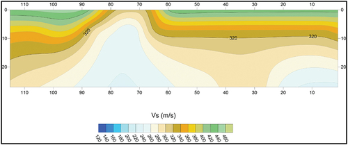
Figure 8. Shear wave velocity depth slice at 32.5m in the study area.

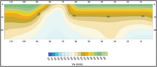
Figure 9. 2D resistivity image inverted from the profile 1 data inverted by the RES2DINV program.

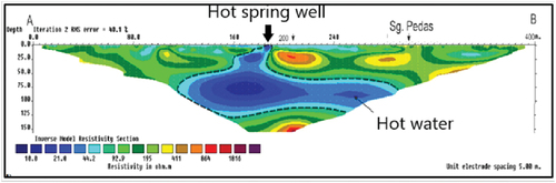
Figure 10. 2D resistivity image inverted from the profile 2 data inverted by the RES2DINV program.

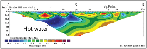
Figure 11. 2D resistivity image inverted from the profile 3 data inverted by the RES2DINV program.

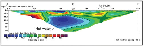
Figure 12. Fence diagram for ERT profiles 1 to 3 in the study area.

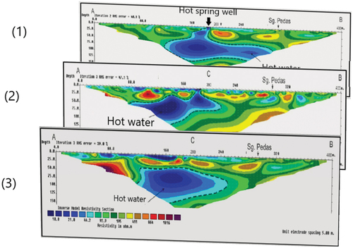
Figure 13. 2D resistivity (above) and chargeability (below) inversion models of the ERT/IP profile 4.

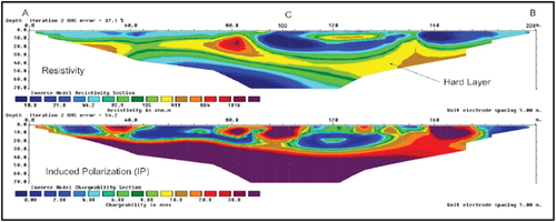
Figure 14. 2D resistivity (above) and chargeability (below) inversion models of the ERT/IP profile 5.

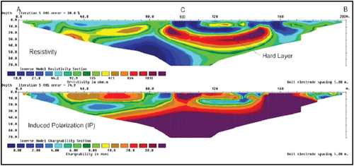
Figure 15. TEM resistivity model in the vicinity of Pedas hot spring.

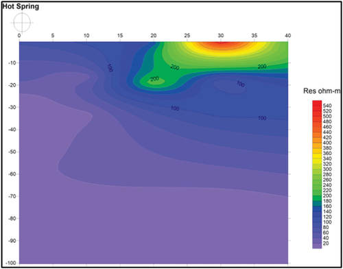
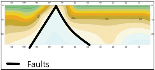
Figure 16. Possible two faults according to geophysical measurements of Pedas hot spring.

Arisona A, Nawawi M, Khalil AE, Nuraddeen UK. 2017. Evaluation study of boundary and depth of the soil structure for geotechnical site investigation using MASW. Journal of Geoscience, Engineering, Environment.

 Google Scholar

Keller George V, Frischknecht Frank C. 1996. Electrical methods in geophysical prospecting:11–23.

 Google Scholar

Murali S, Patangay N. 2006. Principles and application of groundwater geophysics. 3rd ed. Hyderabad: Association of Exploration Geophysicists.

 Google Scholar