Integrated GPR analysis and numerical modelling for discovering archaeological mysteries at Kom Ombo temple

Figures & data

Figure 1. Google earth image shows location of the Kom Ombo temple in the south of Egypt.

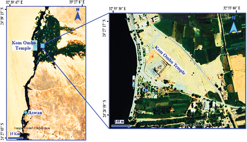
Figure 2. Sketch illustrates (a) GPR survey using GSSI system with 270 MHz central frequency shielded antenna, (b) the distribution of temple’s Zones and GPR survey layout.

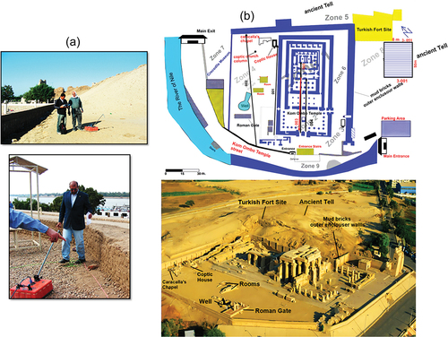
Figure 3. Processing sequence of GPR data along profile (001) at Zone (a), (a) Raw data of 80 MHz central frequency antenna, (b) time zero adjustment, (c) background removal and frequency filters, (d) energy decay and running average, (e) diffraction stack.

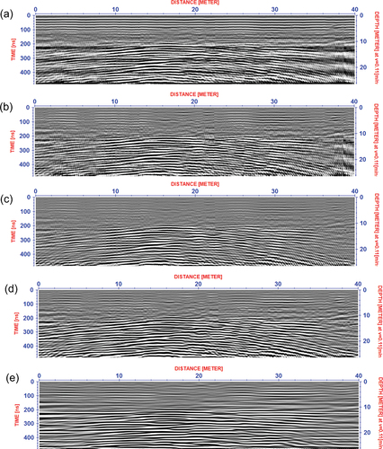
Figure 4. Parallel GPR sections of NE part of Kom Ombo temple represent some reflection events such as (A) hyperbola of extension of Turkish fort mud bricks walls, (B) stratigraphic strata and (C) host medium of silty sand.

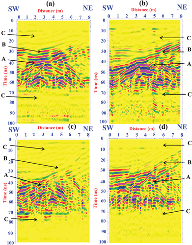
Figure 5. Time slices illustrate the geometry of Turkish fort mud bricks walls, (B) stratigraphic strata and (C) host medium of silty sand.

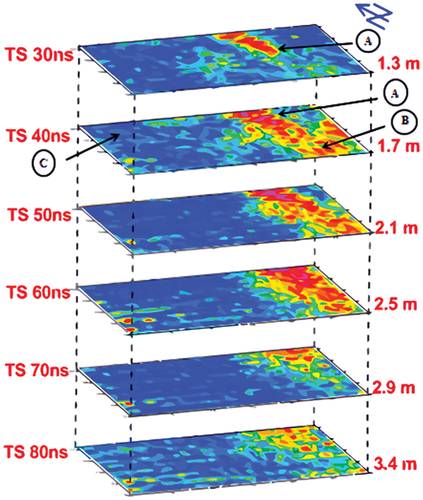
Figure 6. (a, b) Processed GPR sections illustrate deep anomaly (D) and host medium of silty sand (C) inside the temple and on its western side.

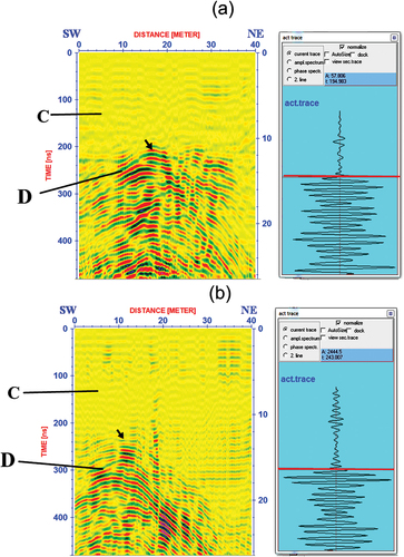
Figure 7. (a) migrated GPR profiles (001, 002) at Zone (4) show anomaly (D) at distance 11 m, depth about 12 m (b) its envelope attribute shows coherent anomaly at distance 11 m and depth about 12 m.

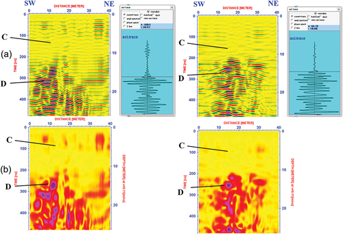
Figure 8. Synthetic model of rectangular geometry.

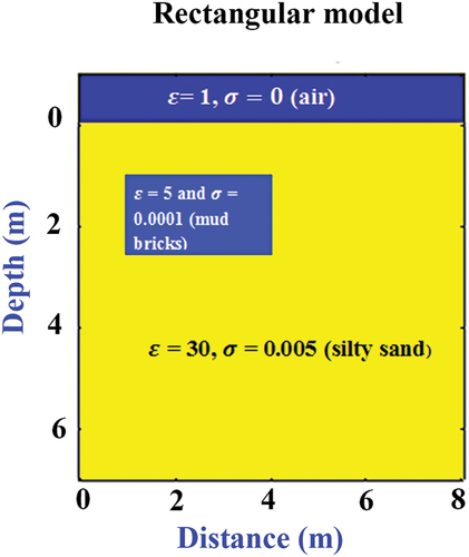
Figure 9. Synthetic model of stepped shape.

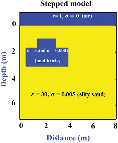
Table 1. Electrical properties of different materials (Davis and Annan 1989; Loke 2015).

No.	Medium	Relative permittivity ε	Electrical conductivity σ (mS/m)	Electromagnetic velocity (m/ns)
1	Air	1	0	0.3
2	Dry sand	3–6	0.1–0.001	0.13–0.17
3	Silty sand	5–30	0.005	0.075
4	Limestone	7–8	0.002–0.00001	0.11
5	Mud bricks	8–40	0.01–1	0.05–0.13

Figure 10. B-scan of rectangular model with high dispersion.

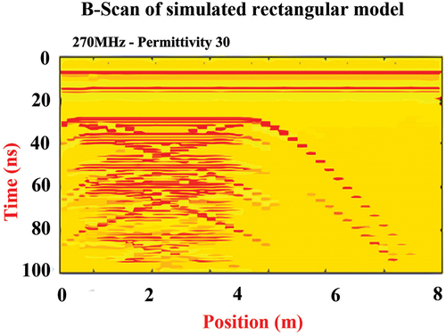
Figure 11. B-scan of low dispersion – simulated rectangular models.

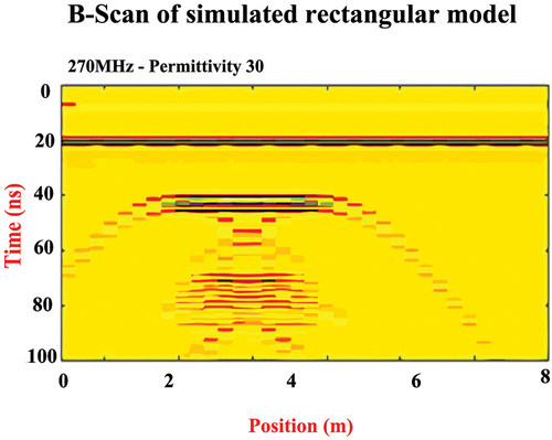
Figure 12. B-Scan of low dispersion- simulated stepped model.

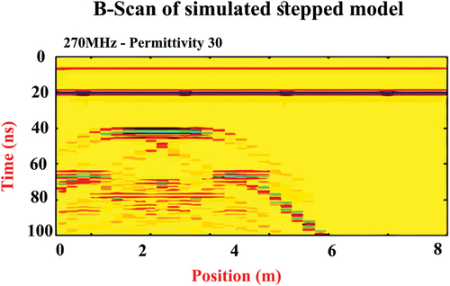
Figure 13. Comparison between (a) GPR section of shallow anomaly and (b) B-scan of low dispersion -simulated rectangular model.

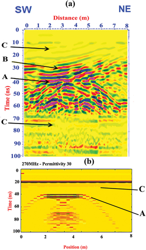
Figure 14. Computational domains of (a) symmetric hyperbola and (b) asymmetric hyperbola models.

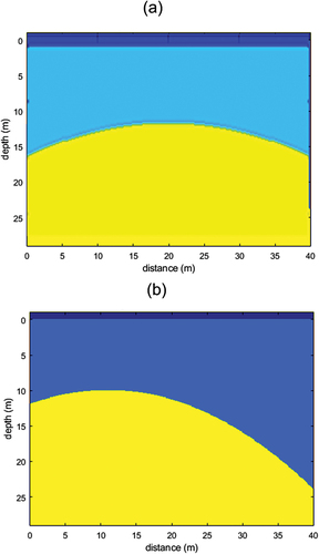
Figure 15. B-scan of the (a) symmetric hyperbola and (b) asymmetric hyperbola models.

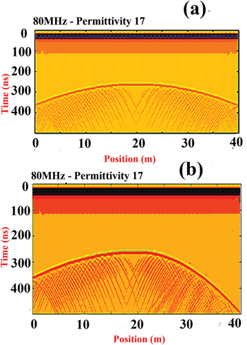
Figure 16. (b) The simulating asymmetric hyperbola model (D) validates (a) deep anomaly (D) under the temple.

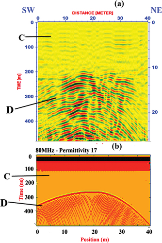
Figure 17. A. symmetrical histogram with a peak near 8.63.

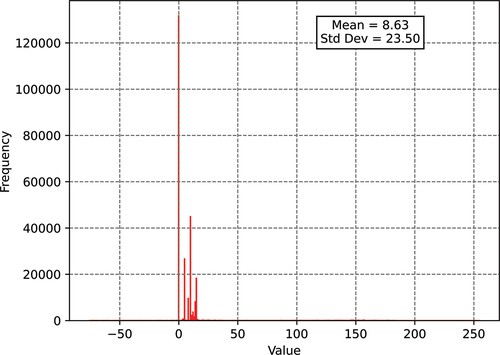
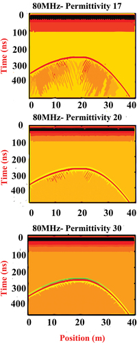
Figure 18. B-Scan from the simulated asymmetric hyperbola model for different values of relative permittivity of silty sand soil.

Davis JL, Annan AP. 1989. Ground-penetrating radar for HIGH-resolution mapping of soil and rock stratigraphy 1. Geophys Prospect. 37(5):531–551. doi: 10.1111/j.1365-2478.1989.tb02221.x.

 Web of Science ®Google Scholar

Loke MH. 2015. Tutorial: 2D and 3D electrical imaging surveys. 4–31.

 Google Scholar