In-use product and steel stocks sustaining the urbanization of Xiamen, China

Figures & data

Figure 1. Geographic location of Xiamen, China

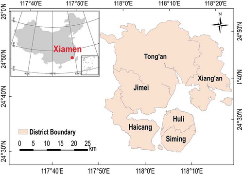
Figure 2. In-use stocks of products in Xiamen during 1980–2015

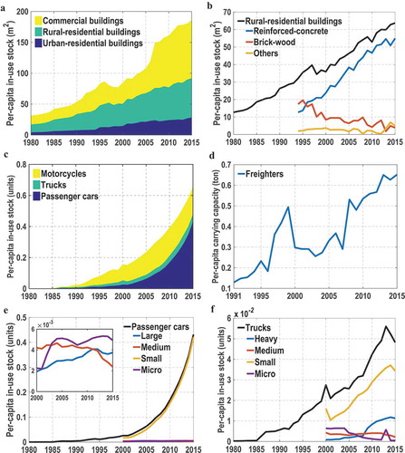
Figure 2. (contined)

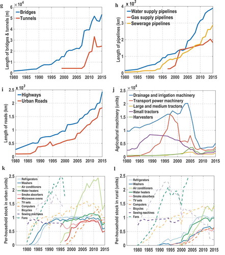
Figure 3. Decomposition of total in-use steel stocks (blue) into five product sectors. Uncertainties of the steel estimation are indicated as bands, with the upper bound, the dark midline, and the lower bound corresponding to the highest, medium, and lowest steel content assumptions. Transportation  = Transportation equipment; Appliances =   Domestic appliances

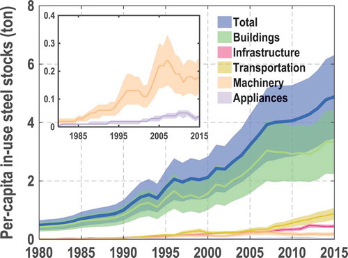
Figure 4. The distribution of in-use steel stocks among end-use sectors during 1980–2015 in Xiamen. Transportation = Transportation equipment; Appliances = Domestic appliances

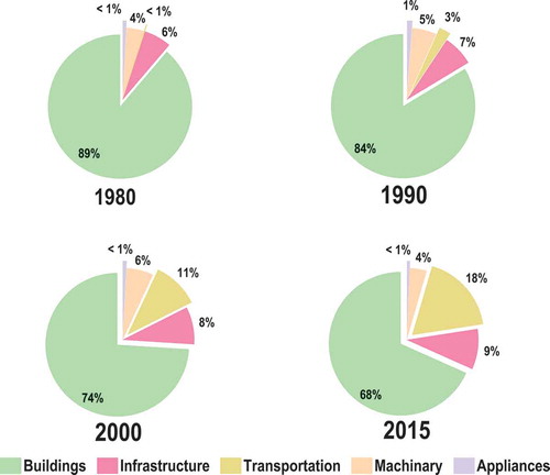
Table 1. Performance of the multiple linear equation

Parameter	Value	R^2	p
a	−5.5	0.99	< 0.001
b1 (Per-capita gross domestic product)	1.7
b2 (Population density)	1.0
b3 (Urban built-up area)	1.8 × 10^−3

Figure 5. The correlations of in-use steel stocks with three socio-economic variables: Per-capita GDP (A), Population density (B), and Urban built-up area (C). The values of GDP are all converted to 2015 constant price

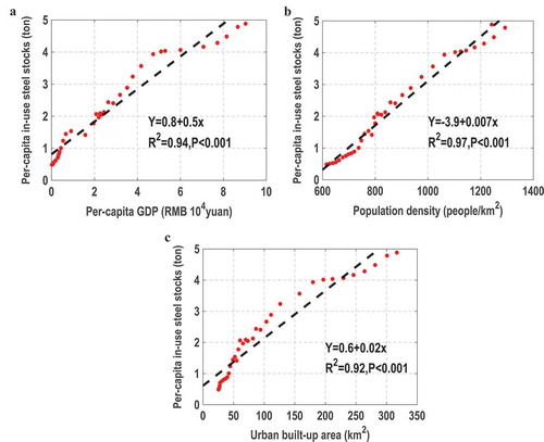
Figure 6. The spatial distribution of in-use steel stocks (t/10⁴m²) in Xiamen for 2000 (A) and 2010 (B)

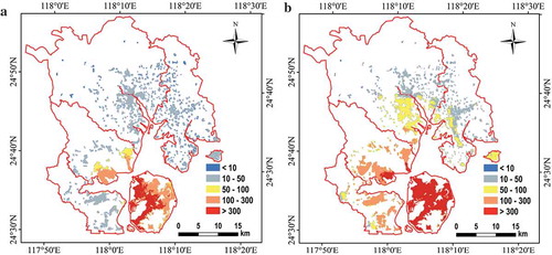
Table A1. Recent studies on in-use steel stocks estimation

Product sectors or categories	Estimation method	Temporal boundary	Spatial boundary	Source
Construction, Transportation, Machinery, Durables, Others	Top-down	2000	Global	Wang, Müller, and Graedel (2007)
Construction, Transportation, Machinery & Appliances, Others	Top-down	1900–2005	Global (Six countries)	Müller, Wang, and Duval (2011)
Building	Top-down	2008	Global	Müller et al. (2013)
Building, Infrastructure, and Others	Top-down	1980–2050	Global	Hatayama, Daigo, and Matsuno (2010)
Building, and Infrastructure	Remote sensing	2012	Global	Liang et al. (2016)
Construction, Machinery, Transportation, Products	Top-down	1700–2008	Global	Pauliuk, Wang, and Müller (2013)
Building, Infrastructure, and Others	Remote sensing	2005	Global	Hsu, Elvidge, and Matsuno (2013)
Passenger cars	Bottom-up	2000–2050	Global	Modaresi et al. (2014)
Construction, Machinery, Automobile, Container, and Others	Top-down	2000	Japan	Daigo et al. (2007)
Construction, Transportation, Container, and Others	Top-down	2002	USA	USGS (2005)
Automobiles	Bottom-up	1970–2001	USA	USGS (2006)
Construction, Transportation, Machinery & Appliances, Others	Top-down	1990–2004	USA	Müller et al. (2006)
Construction, Transportation, Machinery, Appliances, and Others	Top-down	2005	USA	Müller, Wang, and Duval (2011)
Building, and Transportation	Remote sensing	1992–2008	China	Liang et al. (2014)
Building	Top-down	1900–2100	China	Hu et al. (2010)
Building, Road, Railway, and Water pipeline	Bottom-up	1978–2008	China	Han and Xiang (2013)
Building, Machinery, Infrastructure, Transportation, and Appliance	Bottom-up	2000, 2010	China	Wang, Müller, and Hashimoto (2015)
Building, Roads, Railway, and Water pipeline	Bottom-up	1978–2013	Beijing, Shanghai, Tianjin, China	Huang, Han, and Chen (2017)
Building, Transportation, and Equipment	Bottom-up	2005	New Haven, USA	Drakonakis et al. (2007)
Building, Transportation, Infrastructure, and Equipment	Bottom-up	2006	Connecticut, USA	Eckelman, Rauch, and Gordon (2007)

Table A2. The steel contents of different products

End-use sectors	Products	Steel content
Buildings	Non-residential buildings	51 ± 15 kg/m^2
	Urban residential buildings	51 ± 15 kg/m^2
	Rural residential buildings, reinforced-concrete	38 ± 16 kg/m^2
	Rural residential buildings, brick-wood	1.0 ± 0.5 kg/m^2
	Rural residential buildings, others	1.0 ± 0.5 kg/m^2
Infrastructure	Expressways	190 ± 40 t/km
	Highways, Class I	1.5 ± 0.7 t/km
	Highways, Class II	0.7 ± 0.3 t/km
	Urban roads	0.070 ± 0.021 t/km
	Bridges	4.2 ± 1.8 t/m
	Tunnels	1.6 ± 0.8 t/m
	Water supply pipelines	90 ± 27 t/km
	Gas supply pipelines	30 ± 9 t/km
	Sewerage pipelines	8.0 ± 2.4 t/km
	Street lamps	1.0 ± 0.3 t/unit
Transportation equipment	Passenger cars, large	7.6 ± 1.3 t/unit
	Passenger cars, medium	3.2 ± 0.6 t/unit
	Passenger cars, small	0.94 ± 0.19 t/unit
	Passenger cars, micro	0.59 ± 0.06 t/unit
	Trucks, heavy	9.2 ± 1.5 t/unit
	Trucks, medium	3.7 ± 0.8 t/unit
	Trucks, light	1.6 ± 0.4 t/unit
	Trucks, micro	0.78 ± 0.12 t/unit
	Motorcycles	0.085 ± 0.030 t/unit
	Trailers	1.5 ± 1.0 t/unit
	Freighters	0.38 ± 0.10 t/DWT
	Others	2.5 ± 0.8 t/unit
Machinery	Large & medium tractors	3.5 ± 0.8 t/unit
	Small tractors	1.2 ± 0.4 t/unit
	Drainage & irrigation machinery	0.4 ± 0.2 t/unit
	Harvesters	2.0 ± 0.4 t/unit
	Transport power machinery	1.0 ± 0.5 t/unit
	Pumps	0.5 ± 0.2 t/unit
Domestic appliances	Urban, refrigerators	30 ± 6 t/1000unit
	Urban, air conditioners	26 ± 6 t/1000unit
	Urban, washing machines	18 ± 4 t/1000unit
	Urban, microwave ovens	8.0 ± 2.5 t/1000unit
	Urban, water heaters	12.0 ± 4.5 t/1000unit
	Urban, smoke absorbers	20 ± 5 t/1000unit
	Urban, TV sets	0.8 ± 0.2 t/1000unit
	Urban, pianos	40 ± 10 t/1000unit
	Urban, computers	1.5 ± 0.6 t/1000unit
	Urban, bicycles	8 ± 3 t/1000unit
	Urban, sewing machines	20 ± 6 t/1000unit
	Urban, fans	0.8 ± 0.2 t/1000unit
	Rural, refrigerators	30 ± 6 t/1000unit
	Rural, air conditioners	26 ± 6 t/1000unit
	Rural, washing machines	18 ± 4 t/1000unit
	Rural, water heaters	12 ± 4.5 t/1000unit
	Rural, smoke absorbers	20 ± 5 t/1000unit
	Rural, TV sets	0.8 ± 0.2 t/1000unit
	Rural, computers	1.5 ± 0.6 t/1000unit
	Rural, bicycles	8 ± 3 t/1000unit
	Rural, sewing machines	20 ± 6 t/1000unit
	Rural, fans	0.8 ± 0.2 t/1000unit

Table A3. Bottom-up estimation of per-capita in-use steel stocks (ton) during 1980–2015

Year	Buildings	Infrastructure	Transportation equipment	Machinery	Domestic appliances	Total stocks
1980	0.42 ± 0.16	0.03 ± 0.00	0.00 ± 0.00	0.02 ± 0.01	0.00 ± 0.00	0.48 ± 0.17
1981	0.44 ± 0.16	0.03 ± 0.01	0.00 ± 0.00	0.02 ± 0.01	0.01 ± 0.00	0.50 ± 0.18
1982	0.46 ± 0.17	0.03 ± 0.01	0.00 ± 0.00	0.02 ± 0.01	0.01 ± 0.00	0.52 ± 0.18
1983	0.49 ± 0.18	0.04 ± 0.01	0.00 ± 0.00	0.02 ± 0.01	0.01 ± 0.00	0.55 ± 0.19
1984	0.54 ± 0.20	0.04 ± 0.01	0.00 ± 0.00	0.02 ± 0.01	0.01 ± 0.00	0.61 ± 0.21
1985	0.62 ± 0.23	0.04 ± 0.01	0.00 ± 0.00	0.03 ± 0.01	0.01 ± 0.00	0.70 ± 0.25
1986	0.65 ± 0.24	0.05 ± 0.01	0.01 ± 0.00	0.03 ± 0.01	0.01 ± 0.00	0.75 ± 0.26
1987	0.67 ± 0.25	0.05 ± 0.01	0.02 ± 0.00	0.04 ± 0.01	0.01 ± 0.00	0.80 ± 0.27
1988	0.70 ± 0.25	0.06 ± 0.01	0.02 ± 0.00	0.05 ± 0.02	0.01 ± 0.00	0.83 ± 0.29
1989	0.74 ± 0.27	0.06 ± 0.01	0.02 ± 0.00	0.05 ± 0.02	0.01 ± 0.00	0.88 ± 0.30
1990	0.84 ± 0.31	0.07 ± 0.01	0.03 ± 0.01	0.06 ± 0.02	0.01 ± 0.00	1.00 ± 0.35
1991	1.00 ± 0.36	0.08 ± 0.01	0.08 ± 0.02	0.06 ± 0.02	0.01 ± 0.00	1.23 ± 0.42
1992	1.19 ± 0.44	0.08 ± 0.01	0.09 ± 0.02	0.06 ± 0.02	0.01 ± 0.00	1.44 ± 0.50
1993	1.25 ± 0.46	0.09 ± 0.01	0.11 ± 0.03	0.06 ± 0.02	0.02 ± 0.00	1.53 ± 0.53
1994	1.10 ± 0.41	0.10 ± 0.01	0.13 ± 0.03	0.07 ± 0.03	0.02 ± 0.00	1.41 ± 0.49
1995	1.40 ± 0.51	0.12 ± 0.01	0.15 ± 0.04	0.09 ± 0.04	0.02 ± 0.00	1.77 ± 0.60
1996	1.66 ± 0.61	0.13 ± 0.02	0.14 ± 0.03	0.11 ± 0.05	0.02 ± 0.01	2.06 ± 0.71
1997	1.43 ± 0.53	0.15 ± 0.02	0.2 ± 0.06	0.13 ± 0.06	0.02 ± 0.00	1.96 ± 0.66
1998	1.52 ± 0.56	0.16 ± 0.02	0.26 ± 0.06	0.13 ± 0.06	0.02 ± 0.00	2.08 ± 0.70
1999	1.41 ± 0.51	0.18 ± 0.03	0.29 ± 0.07	0.13 ± 0.05	0.02 ± 0.01	2.04 ± 0.67
2000	1.57 ± 0.57	0.18 ± 0.03	0.22 ± 0.05	0.13 ± 0.05	0.02 ± 0.00	2.12 ± 0.71
2001	1.88 ± 0.67	0.21 ± 0.03	0.21 ± 0.05	0.11 ± 0.04	0.02 ± 0.01	2.43 ± 0.81
2002	1.81 ± 0.66	0.23 ± 0.03	0.23 ± 0.05	0.11 ± 0.04	0.02 ± 0.01	2.40 ± 0.79
2003	2.03 ± 0.71	0.23 ± 0.03	0.23 ± 0.05	0.14 ± 0.06	0.03 ± 0.01	2.66 ± 0.86
2004	2.18 ± 0.76	0.23 ± 0.03	0.26 ± 0.06	0.18 ± 0.08	0.03 ± 0.01	2.88 ± 0.93
2005	2.42 ± 0.85	0.26 ± 0.03	0.30 ± 0.07	0.22 ± 0.08	0.03 ± 0.01	3.23 ± 1.04
2006	2.72 ± 0.92	0.25 ± 0.03	0.34 ± 0.08	0.22 ± 0.08	0.04 ± 0.01	3.56 ± 1.12
2007	3.04 ± 1.04	0.26 ± 0.03	0.34 ± 0.08	0.24 ± 0.09	0.04 ± 0.01	3.93 ± 1.25
2008	2.99 ± 1.03	0.30 ± 0.04	0.45 ± 0.11	0.22 ± 0.08	0.04 ± 0.01	4.01 ± 1.28
2009	2.98 ± 0.98	0.33 ± 0.05	0.48 ± 0.11	0.19 ± 0.07	0.04 ± 0.01	4.03 ± 1.22
2010	2.92 ± 0.96	0.34 ± 0.05	0.56 ± 0.13	0.19 ± 0.07	0.05 ± 0.01	4.06 ± 1.21
2011	2.96 ± 0.97	0.36 ± 0.06	0.63 ± 0.14	0.16 ± 0.06	0.05 ± 0.01	4.16 ± 1.24
2012	2.91 ± 0.96	0.47 ± 0.06	0.68 ± 0.15	0.18 ± 0.06	0.05 ± 0.01	4.28 ± 1.25
2013	3.05 ± 1.00	0.46 ± 0.06	0.76 ± 0.17	0.18 ± 0.06	0.04 ± 0.01	4.48 ± 1.31
2014	3.33 ± 1.08	0.44 ± 0.05	0.81 ± 0.18	0.17 ± 0.06	0.03 ± 0.01	4.78 ± 1.39
2015	3.34 ± 1.10	0.45 ± 0.06	0.88 ± 0.20	0.18 ± 0.06	0.04 ± 0.01	4.88 ± 1.43

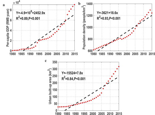
Figure A1. Patterns of three socio-economic factors in Xiamen during 1980–2015. Per-capita GDP (A), Population density (B), and Urban built-up area (C). The values of GDP (RMB yuan) are all converted to 2015 constant price

Wang, T., D. B. Müller, and T. E. Graedel. 2007. “Forging the Anthropogenic Iron Cycle.” Environmental Science & Technology 41 (14): 5120–5129. doi:10.1021/es062761t.

 Google Scholar

Müller, D. B., T. Wang, and B. Duval. 2011. “Patterns of Iron Use in Societal Evolution.” Environmental Science & Technology 45 (1): 182–188. doi:10.1021/es102273t.

 Google Scholar

Müller, D. B., G. Liu, A. N. Løvik, R. Modaresi, S. Pauliuk, F. S. Steinhoff, and H. Brattebø. 2013. “Carbon Emissions of Infrastructure Development.” Environmental Science & Technology 47: 11739–11746. doi:10.1021/es402618m.

 Google Scholar

Hatayama, H., I. Daigo, and Y. Matsuno. 2010. “Outlook of the World Steel Cycle Based on the Stock and Flow Dynamics.” Environmental Science & Technology 44: 6457–6463. doi:10.1021/es100044n.

 Google Scholar

Liang, H., L. Dong, H. Tanikawa, N. Zhang, Z. Gao, and X. Luo. 2016. “Feasibility of a New-Generation Nighttime Light Data for Estimating In-Use Steel Stock of Buildings and Civil Engineering Infrastructures.” Resources, Conservation and Recycling 123: 11–23. doi:10.1016/j.resconrec.2016.04.001.

 Google Scholar

Pauliuk, S., T. Wang, and D. B. Müller. 2013. “Steel All over the World: Estimating In-Use Steel Stocks of Iron for 200 Countries.” Resources, Conservation and Recycling 71 (1): 22–30. doi:10.1016/j.resconrec.2012.11.008.

 Google Scholar

Hsu, F., C. D. Elvidge, and Y. Matsuno. 2013. “Exploring and Estimating In-Use Steel Stocks in Civil Engineering and Buildings from Night-Time Lights.” International Journal of Remote Sensing 34 (2): 490–504. doi:10.1080/01431161.2012.712232.

 Google Scholar

Modaresi, R., S. Pauliuk, A. N. Løvik, and D. B. Müller. 2014. “Global Carbon Benefits of Materials Substitution in Passenger Cars Until 2050 and The Impact on The Steel and Aluminum Industries.” Environmental Science & Technology 48 (18): 10776–10784.

 Google Scholar

Daigo, I., Y. Igarashi, Y. Matsuno, and Y. Adachi. 2007. “Accounting for Steel Stock in Japan.” ISIJ International 47 (7): 1065–1069. doi:10.2355/isijinternational.47.1065.

 Google Scholar

USGS. 2005. Metal Stocks in Use in the United States. Denver, CO: USGS.

 Google Scholar

USGS. 2006. Steel Stocks in Use in Automobiles in the United States. Buckingham, D.A: USGS.

 Google Scholar

Müller, D. B., T. Wang, B. Duval, and T. E. Graedel. 2006. “Exploring the Engine of Anthropogenic Iron Cycles.” Proceedings of the National Academy of Sciences of the United States of America 103 (44): 16111–16116. doi:10.1073/pnas.0603375103.

 Google Scholar

Liang, H., H. Tanikawa, Y. Matsuno, and L. Dong. 2014. “Modeling In-Use Stock in China’s Building and Civil Engineering Infrastructure Using Time-Series of DMSP/OLS Nighttime Lights.” Remote Sensing 6: 4780–4800. doi:10.3390/rs6064780.

 Google Scholar

Hu, M., S. Pauliuk, T. Wang, G. Huppes, E. V. Der Voet, and D. B. Müller. 2010. “Iron and Steel in Chinese Residential Buildings: A Dynamic Analysis.” Resources Conservation and Recycling 54 (9): 591–600. doi:10.1016/j.resconrec.2009.10.016.

 Google Scholar

Han, J., and W. N. Xiang. 2013. “Analysis of Material Stock Accumulation in China’s Infrastructure and Its Regional Disparity.” Sustainability Science 8 (4): 553–564. doi:10.1007/s11625-012-0196-y.

 Google Scholar

Wang, T., D. B. Müller, and S. Hashimoto. 2015. “The Ferrous Find: Counting Iron and Steel Stocks in China’s Economy.” Journal of Industrial Ecology 19 (5): 877–889. doi:10.1111/jiec.12319.

 Google Scholar

Huang, C., J. Han, and W. Q. Chen. 2017. “Changing Patterns and Determinnants of Infrastructures’ Material Stocks in Chinese Cities.” Resources, Conservation and Recycling 123: 47–53. doi:10.1016/j.resconrec.2016.06.014.

 Google Scholar

Drakonakis, K., K. H. Rostkowski, J. N. Rauch, T. E. Graedel, and R. B. Gordon. 2007. “Metal Capital Sustaining a North American City: Iron and Copper in New Haven, CT.” Resources Conservation and Recycling 49 (4): 406–420. doi:10.1016/j.resconrec.2006.05.005.

 Google Scholar

Eckelman, M. J., J. Rauch, and R. B. Gordon. 2007. “In-Use Stocks of Iron in the State of Connecticut, USA.” Working Paper Number 11. New Haven, CT: Scholl of Forestry and Environmental Studies, Yale University. doi:10.1094/PDIS-91-4-0467B.

 Google Scholar