Linking observation, modelling and satellite-based estimation of global land evapotranspiration

Figures & data

Figure 1. Evapotranspiration includes plant transpiration, canopy interception evaporation, and soil evaporation (downloaded from https://science.nasa.gov/earth-science/oceanography/ocean-earth-system/ocean-water-cycle/).

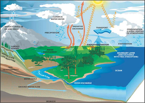
Figure 2. Land evapotranspiration consists of transpiration from vegetation and evaporation from water day, wet leaf, and soil.

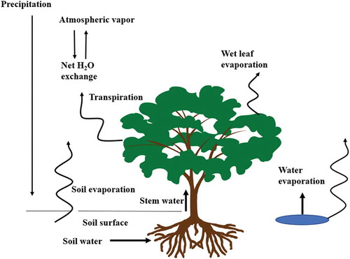
Figure 3. A map of FLUXNET sites and climate (Koppen-Geiger classification) (Figure is adopted from Wang & Dickinson (2012), i.e. downloaded from http://www.fluxnet.ornl.gov/fluxnet/graphics.cfm).

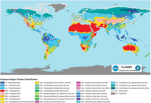
Figure 4. Summary of tower sites that are registered in FLUXNET (closed bars) and included in the FLUXNET2015 Dataset (open bars). “Registered sites” represent sites that have been registered in fluxdata.org, FLUXNET-ORNL, AmeriFlux, ICOS, AsiaFlux, OzFlux, or ChinaFlux. Sites are grouped by regions (b-g) and vegetation classification (h-n) (IGBP: International Geosphere–Biosphere Programme). Forest: ENF+DBF+EBF+MF, Grassland: GRA, Cropland: CRO+CVM, Wetland: WET, Shrubland: OSH+CSH, Savanna: SAV+WSA, Other: BSV+URB+WAT+SNO (last updated in February 2017) (figure downloaded from https://fluxnet.fluxdata.org/sites/site-summary/).

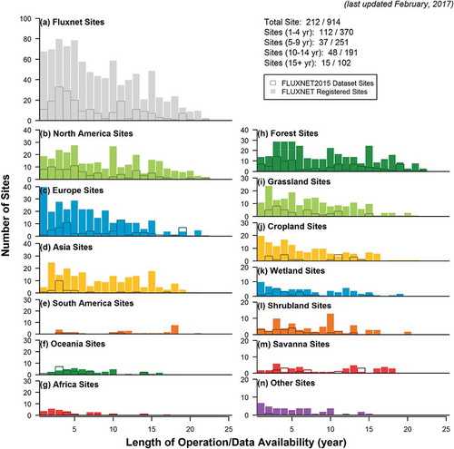
Figure 5. Distribution of FLUXNET sites across temperature and precipitation ranges (a.k.a., Whittaker’s biome classification), compared to land surface from the terrestrial globe. The length of the record of sites is represented in the circle sizes and colors (a-c). Panel (a) shows the sites included in the La Thuile 2007 Dataset; panel (b) shows the sites included in the FLUXNET2015 Dataset; panel (c) shows all sites present in FLUXNET; and, panel (d) compares the distribution of land surface, FLUXNET sites, and sites in the FLUXNET2015 Dataset across these temperature-precipitation ranges. (Pastorello et al., 2017, EOS) (Figure downloaded from https://fluxnet.fluxdata.org/about/).

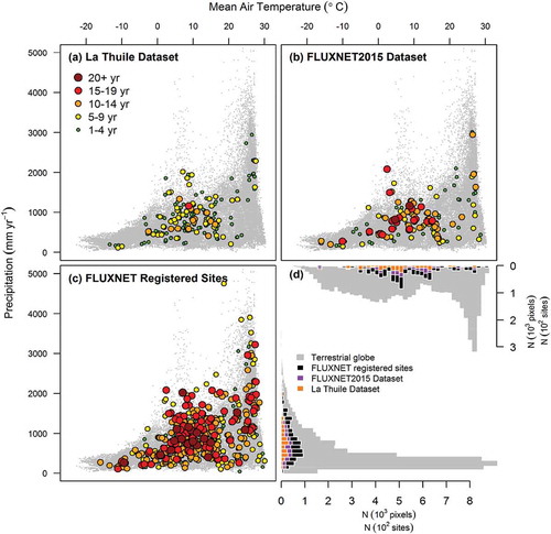
Figure 6. Global evapotranspiration (mm d⁻²) for a single day at 1 km resolution for PT-JPL from MODIS (Fisher, 2018).

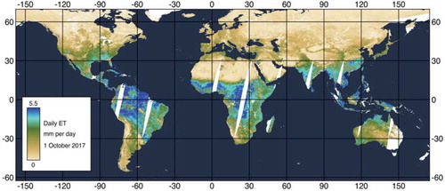
Figure 7. The spatial patterns of the mean annual AET with MTE observation, BESS and MODIS estimates over 2001–2011.

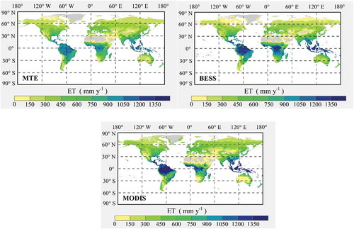
Figure 8. The error in ET estimates for the PT-JPL model is sensitive to driving variable errors, adopted from Fisher et al., 2017).

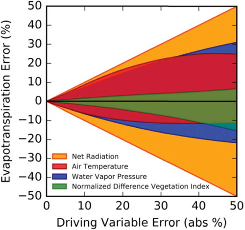
Figure 9. Flow chart showing data processing stream for the PT-JPL _SM model (Purdy et al., 2018).

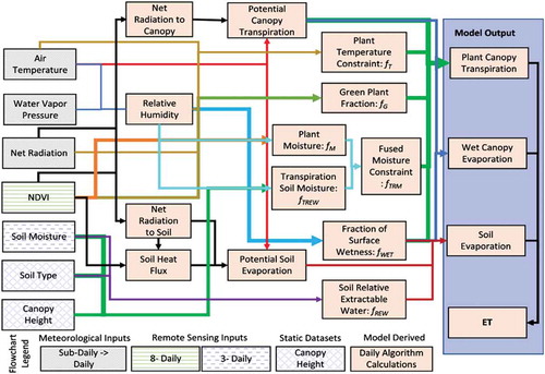
Figure 10. Evapotranspiration components as expressed as a percentage of total ET. Red indicates more soil evaporation, blue indicates more transpiration, yellow indicates more canopy interception evaporation. Below, total contribution to annual ET from transpiration, soil evaporation, and interception (Modified from Purdy et al., 2018).

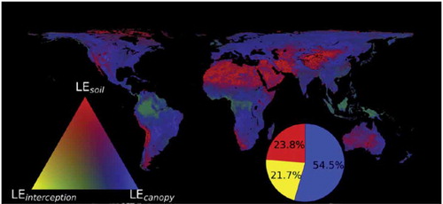
Figure 11. Water budget processes of cropland in the RS-WBPM2 model, where F⁽¹⁾ denotes the water infiltrated from the soil surface to soil layer (1), F⁽²⁾ and F⁽³⁾ denote the water percolated from the upper layer to soil layers (2) and (3), respectively, and swl_a ⁽¹⁾, swl_a ⁽²⁾, and swl_a ⁽³⁾ denote the water loss of soil layers (1), (2), and (3), respectively, by transpiration (E_dry ^c) (Bai et al., 2018).

Table 1. Summarize for the global ET estimates.

No.	Models	Period	Annual $ET$ (${10}^3\mathrm{k}{\mathrm{m}}^3$)	Trend$(\mathrm{m}\mathrm{m}/\mathrm{a})$	Reference
1	Empirical Eq.	1986–1995	47.5$\mathrm{W}/{\mathrm{m}}^2$	-	(Wang & Liang, 2008)
2	MTE	1982–2008	65$\pm$3	1982–1997: 0.71 1998–2008: -0.16 Overall: 0.41	(Jung et al., 2010)
3	Two-Source PM	1984–1998	58.4	1.55	(Yan et al., 2012)
4	Two-Source PM	1982–2011	64.8$\pm$0.8	1982–1997: 0.4 1998–2008: -0.2 Overall: 0.46	(Yan et al., 2013)
5	Semi-Empirical TP	2003–2005	41.7$\mathrm{W}/{\mathrm{m}}^2$	-	(Yao et al., 2015)
6	Two-Source PM	2000–2006	62.8	-	(Mu et al., 2011)
7	Corrected PT	1986–1993	-	$\uparrow$	(Fisher et al., 2008)

Figure 12. Distribution of global trend of ARTS ensemble average ET and its significance of linear trend for period of (a, b) 1982–2011, (c, d) 1982–1997, and (e, f) 1998–2011, respectively (Yan et al., 2013).

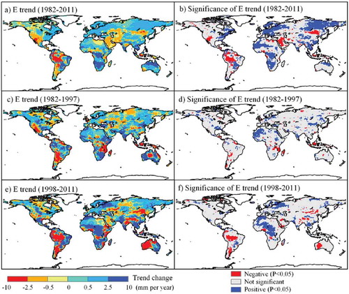
Figure 13. Soil-moisture and ET trends. Significant (P,0.1) soil-moisture trends derived from TRMM (a), significant (P,0.1) ET trends from MTE (b) and mean ET and soil-moisture anomalies (seasonal cycle subtracted and filtered with an 11-month running mean) of all valid pixels of the TRMM domain (c). For consistency and improved comparability, regions without data in either MTE (non-vegetated areas) or TRMM soil-moisture data (very dense vegetation) are blanked in the trend maps of a and b. (Jung et al., 2010).

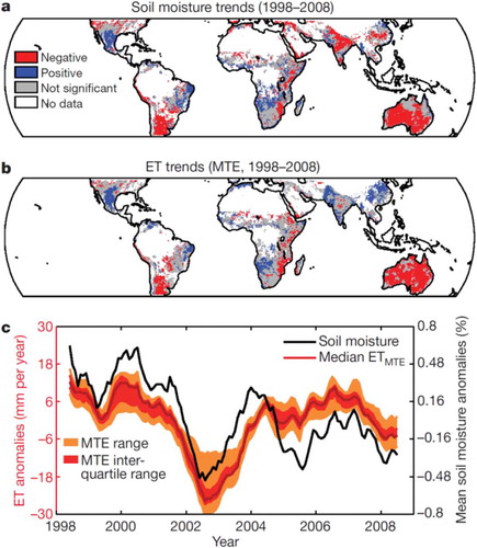
Figure 14. A schematic of an ecosystem experiment designed to measure transpiration and evaporation from soil and intercepted water using multiple complementary measurement approaches (Stoy et al., 2019).

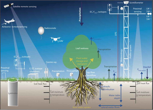
Table A1. Variables symbol list in this paper.

Variables Symbol	Meanings
ET	Evapotranspiration
AET	Actual evapotranspiration
$\lambda E$	Latent heat flux
$\lambda E_{wet}$	Latent heat without water stress
$\lambda E_c$	Latent heat flux from the vegetation canopy
$\lambda E_s$	Latent heat flux from the soil surface
H	sensible heat flux
G	Ground heat flux
Rn	Surface net radiation
$R_g$	Surface global solar radiation
$R_e$	Extra solar radiation for a given day and a given position on the earth
E	Evaporation
T	Transpiration
Ta	Air temperature
$\mathrm{\Delta }{T}_a$	Vertical air temperature difference
T0	Aerodynamic temperature
Ts	Land surface temperature
$\mathrm{\Delta }{T}_s$	day–night Ts difference
Tc	canopy temperature
$T^{\ast }$	Temperature scale
DTsR	Diurnal land surface or air temperature range
$r_0$	Fractional hemispheric surface reflectance
$r_a$	Aerodynamic resistance
$r_s$	Surface resistance
$r_{bl}$	Boundary layer resistance
$\rho$	Air density
$c_p$	Air constant pressure specific heat
$C$	Regression coefficient related with soil condition
$a$	Regression coefficient
$a_i,i=0,1,\mathrm{2..}n$	Regression coefficient
$b$	Regression coefficient
$K_c$	Ratio of soil heat flux to net radiation for full canopy
$K_s$	Ratio of soil heat flux to net radiation with bare soil
$k{B}^{-1}$	Calculating air resistance to heat transport
$\mathrm{\Delta }$	Water vapor pressure gradient
$\gamma$	Psychrometric constant
${\mathrm{e}}_s$	Saturation vapour pressure
${\mathrm{e}}_a$	Actual water vapor pressure
$\alpha$	Priestley-Taylor coefficient controlled by surface water condition
${\mathrm{g}}_s$	Surface conductance
${\mathrm{c}}_L$	Mean surface conductance per unit leaf area index
${\mathrm{g}}_{s,min}$	Surface conductance controlling soil evaporation and the conductance through the leaf cuticle (Cleugh et al., 2007)
gst	Stomatal conductance
gsmax	Optimum stomatal conductance
$G_c$	Canopy conductance
VPD	Vapor pressure deficit
VI	Vegetation index
$NDVI$	Normalized difference vegetation index
EVI	Enhanced vegetation index
CWSI	Crop water stress index
SAVI	Soil adjusted vegetation index
LAI	Leaf area index
$f\left(C\right)$	Fractional canopy cover
VFC	Vegetation fractional cover
fAPAR	Fraction of Absorbed Photosynthetically Active Radiation
BRDF	Bidirectional Reflectance Distribution Function
RH	Relative humidity
SM	Soil moisture

Wang, K., & Dickinson, R. E. (2012). A review of global terrestrial evapotranspiration: Observation, modeling, climatology, and climatic variability. Reviews of Geophysics, 50(2). doi:10.1029/2011rg000373

 Google Scholar

Pastorello, G. Z., Papale, D., Chu, H., Trotta, C., Agarwal, D., Canfora, E., … Torn, M. (2017). A new data set to keep a sharper eye on land-air exchanges. EOS, Transactions American Geophysical Union, 98. doi:10.1029/2017EO071597

 Google Scholar

Fisher, J. B., and ECOSTRESS Algorithm Development Team (2018). ECOsystem Spaceborne Thermal Radiometer Experiment on Space Station (ECOSTRESS): Level-3 Evapotranspiration LE(ET_PT-JPL) Algorithm Theoretical Basis Document (ATBD). ECOSTRESS Science Document no. D-94645. Jet Propulsion Laboratory, Pasadena.

 Google Scholar

Fisher, J. B., Melton, F., Middleton, E., Hain, C., Anderson, M., Allen, R., & Wood, E. F. (2017). The future of evapotranspiration: Global requirements for ecosystem functioning, carbon and climate feedbacks, agricultural management, and water resources. Water Resources Research, 53(4), 2618–2626.

 Web of Science ®Google Scholar

Purdy, A. J., Fisher, J. B., Goulden, M. L., Colliander, A., Halverson, G., Tu, K., & Famiglietti, J. S. (2018). SMAP soil moisture improves global evapotranspiration. Remote Sensing of Environment, 219, 1–14.

 Web of Science ®Google Scholar

Bai, Y., Zhang, J., Zhang, S., Yao, F., & Magliulo, V. (2018). A remote sensing-based two-leaf canopy conductance model: Global optimization and applications in modeling gross primary productivity and evapotranspiration of crops. Remote Sensing of Environment, 215, 411–437.

 Web of Science ®Google Scholar

Wang, K., & Liang, S. (2008). An improved method for estimating global evapotranspiration based on satellite determination of surface net radiation, vegetation index, temperature, and soil moisture. Journal of Hydrometeorology, 9(4), 712–727.

 Web of Science ®Google Scholar

Jung, M., Reichstein, M., Ciais, P., Seneviratne, S. I., Sheffield, J., Goulden, M. L., … Zhang, K. (2010). Recent decline in the global land evapotranspiration trend due to limited moisture supply. Nature, 467(7318), 951–954.

 PubMed Web of Science ®Google Scholar

Yan, H., Wang, S. Q., Billesbach, D., Oechel, W., Zhang, J. H., Meyers, T., … Scott, R. (2012). Global estimation of evapotranspiration using a leaf area index-based surface energy and water balance model. Remote Sensing of Environment, 124, 581–595.

 Web of Science ®Google Scholar

Yan, H., Yu, Q., Zhu, Z., Myneni, R. B., Yan, H., Wang, S., & Shugart, H. H. (2013). Diagnostic analysis of interannual variation of global land evapotranspiration over 1982–2011: Assessing the impact of ENSO. Journal of Geophysical Research: Atmospheres, 118(16), 8969–8983.

 Web of Science ®Google Scholar

Yao, Y., Liang, S., Li, X., Chen, J., Wang, K., Jia, K., … Roupsard, O. (2015). A satellite-based hybrid algorithm to determine the Priestley–Taylor parameter for global terrestrial latent heat flux estimation across multiple biomes. Remote Sensing of Environment, 165, 216–233.

 Web of Science ®Google Scholar

Mu, Q., Zhao, M., & Running, S. W. (2011). Improvements to a MODIS global terrestrial evapotranspiration algorithm. Remote Sensing of Environment, 115(8), 1781–1800.

 Web of Science ®Google Scholar

Fisher, J. B., Tu, K. P., & Baldocchi, D. D. (2008). Global estimates of the land–atmosphere water flux based on monthly AVHRR and ISLSCP-II data, validated at 16 FLUXNET sites. Remote Sensing of Environment, 112(3), 901–919.

 Web of Science ®Google Scholar

Stoy, P. C., El-Madany, T. S., Fisher, J. B., Gentine, P., Gerken, T., Good, S. P., … Wolf, S. (2019). Reviews and syntheses: Turning the challenges of partitioning ecosystem evaporation and transpiration into opportunities. Biogeosciences, 16(19), 3747–3775.

 Web of Science ®Google Scholar

Cleugh, H. A., Leuning, R., Mu, Q., & Running, S. W. (2007). Regional evaporation estimates from flux tower and MODIS satellite data. Remote Sensing of Environment, 106(3), 285–304.

 Web of Science ®Google Scholar