A 100 m population grid in the CONUS by disaggregating census data with open-source Microsoft building footprints

Figures & data

Table 1. Summary of existing population grid products in different geographic regions

Grid population datasets	Grid size	Location(s) and year(s) represented	Input variable(s)	Methods	Source
History Database of the Global Environment (HYDE) Population Grids, version 3.1 (Klein Goldewijk, Beusen, Van Drecht, & De Vos, 2011)	5 arc-minutes (10 km)	Global, 10,000 BC to 2000 AD	Historical population, croplands, and pasture	Spatially explicit allocation mapping.	Netherlands Environmental Assessment Agency (PBL)
Gridded Population of the World (GPW), version 4 (latest version) (Doxsey-Whitfield et al., 2015)	30 arc-seconds (1 km)	Global, 2000, 2005, 2010, 2015, 2020	Census population, protected areas, water bodies	Areal weighting method that assumes population is uniformly distributed for habitable cells covering census units.	Center for International Earth Science Information Network (CIESIN), Columbia University
Global Rural Urban Mapping Project (GRUMP) (Balk et al., 2006)	30 arc-seconds (1 km)	Global, 1990, 1995, 2000	Census population, protected area, water bodies, urban boundaries, nighttime lights (DMSP)	Binary dasymetric method that uses nighttime lights to allocate population in urban areas.	CIESIN, Columbia University
Global Human Settlement – Population (GHS-POP) (Freire & Pesaresi, 2015)	30 arc-seconds (1 km) and 9 arc-seconds (250 m)	Global 1975, 1990, 2000, 2015	Census population, urban areas from Landsat imagery	Binary dasymetric method that uses Landsat imagery to allocate population in urban areas.	European Commission Joint Research Centre (JRC) and CIESIN, Columbia University
LandScan Global Population Database (Dobson, Bright, Coleman, Durfee, & Worley, 2000)	30 arc-seconds (1 km)	Global, Annual release from 2000–2017 (current)	Census population, roads, land cover, urban areas, environmental variables, water bodies	Dasymetric method that uses land cover, imagery-derived urban areas, and multiple environmental variables to allocate population inhabitable cells.	Oak Ridge National Laboratory (ORNL)
World Population Estimate (WPE) (Frye et al., 2018)	5 arc-seconds (150 m) after 2016, 8 arc-seconds (250 m) before 2016	Global, 2013, 2015, 2016 (current)	Census population, land cover, road, water bodies	Dasymetric method that uses land cover, road density to allocate population inhabitable cells.	ESRI
WorldPop (Tatem, 2017)	30 arc-seconds (1 km) for global mosaic, 3 arc-second (100 m) for all countries in the world	Selected countries (the US excluded), represented year is country-specific	Census population, land cover, roads, urban area, nighttime lights, environment variables, protected areas, water bodies	Dasymetric mapping method that uses statistical weighting layer derived from machine learning approach (Random Forest) to allocate population inhabitable cells	WorldPop
Gridded Population Mapping (Demobase) (Azar, Engstrom, Graesser, & Comenetz, 2013)	3 arc-second (100 m)	Selected countries (Haiti, Pakistan, and Rwanda), represented year is country-specific	Census population, environmental variables, impervious surface from Landsat imagery	Dasymetric mapping method that uses Landsat-derived impervious surface and other environmental variables to allocate population inhabitable cells.	US Census Bureau
High Resolution Settlement Layer (HRSL) (Tiecke et al., 2017)	1 arc-second (30 m)	Selected countries (33 in total, US excluded), 2015	Census population, high resolution imagery (0.5 m) from DigitalGlobe	Binary dasymetric method that uses image-derived building footprints to allocate population in cells with building footprints.	Facebook Connectivity Lab and CIESIN
WSF-POP (Palacios-Lopez et al., 2019)	10 m	Global 2015	Census data, WSF-2015 Layer (binary human settlement layer), WSF-2015-Density (percent impervious surface layer)	Dasymetric mapping method that uses binary human settlement or percent impervious surface to allocate population in habitable cells.	German Aerospace Center (DLR)
OpenPopGrid (Murdock, Harfoot, Martin, Cockings, & Hill, 2015)	10 m	England, UK and Wales, UK, 2011	Census postcode headcounts, postcode centroids, building footprints	Binary dasymetric method that uses building footprints classified by postcode centroid to allocate population in cells with building footprints.	GeoData, University of Southampton

Figure 1. Distribution of microsoft building footprints and example sites (grey polygons) in the CONUS

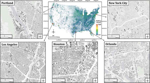
Table 2. OSM land-use statistics in the CONUS

Land-use class	Total records	Total size ($k{m}^2$)	Land-use class	Total records	Total size ($k{m}^2$)
Allotments	1,681	4.52	Industrial	52,537	9,079.45
Commercial	64,216	2,949.86	Meadow	42,615	23,430.72
Farm	186,297	73,989.69	Military	3,124	112,921.92
Forest	358,426	274,690.80	Natural reserve	27,215	683,926.68
Grass	262,348	2,356.47	Orchard	18,259	3583.34
Park	124,472	34,573.64	Quarry	7119	4,197.45
Recreation Ground	21,545	3,238.34	Residential	373,261	42,348.51
Retail	42,913	2,164.11	Scrub	62,416	13,940.30
Vineyard	15,137	1,847.07	Cemetery	45,904	1,529.74
Health	4,587	16,063.60

Note. OSM data used in this study was downloaded on March 1^st, 2019.

Table 3. Six metrics of statistical measures used for accuracy assessment

Name and abbreviation	Equation
Root mean square error (RMSE)	$RMSE=\sqrt{\frac{{\sum }_{j=1}^n{\left(P_j^e-P_j^g\right)}^2}{n}}$
Mean absolute error (MAE)	$MAE=\frac{{\sum }_{j=1}^n\left|P_j^e-P_j^g\right|}{n}$
Overall relative error (ORE)	$ORE=\frac{{\sum }_{j=1}^n\left|\frac{P_j^e-P_j^g}{P_j^g}\right|}{n}\times 100\mathrm{\%}$
Coefficient of efficiency (CoE)	$CoE=1-\frac{{\sum }_{j=1}^n{\left(P_j^g-P_j^e\right)}^2}{{\sum }_{j=1}^n{\left(P_j^g-\overline{P_j^g}\right)}^2}$
Systematic error (SE)	$SE=\frac{{\sum }_{j=1}^n{P}_j^e-P_j^g}{n}$
Modified index of agreement (IoA)	$MIoA=1-\frac{{\sum }_{j=1}^n|P_j^g-P_j^e|}{{\sum }_{j=1}^n\left(\left|P_j^e-\overline{P_j^g}\right|+\left|P_j^g-\overline{P_j^g}\right|\right)}$

Note. $P_j^e$ and $P_j^g$ denote the extracted population and ACS ground population in block group $j,$ respectively. $\overline{P_j^g}$ denotes the mean true population in all block groups.

Figure 2. Example population grids before and after trimming in Addison, TX. (a) Original building footprints; (b) OSM crowdsourced land-use types; (c) trimmed building footprints; (d) population grid weighted with original building footprint size; (e) population grid weighted with trimmed building footprint size

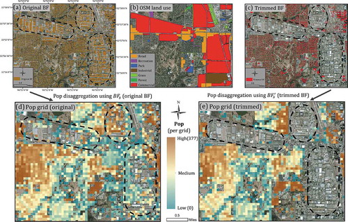
Table 4. Performance evaluation of the four weighting scenarios

Scenarios	RMSE	MAE	ORE	SE	CoE	MIoA
$B{F}_c^{\prime }$	480.96	313.53	26.24%	3.52	0.75	0.75
$B{F}_s^{\prime }$	444.43	298.74	25.55%	3.51	0.79	0.76
$B{F}_{sc}^{\prime }$	490.06	320.38	26.44%	3.54	0.74	0.75
UNIF	1102.57	606.75	52.08%	37.96	−0.32	0.58

Note. The best performance for each individual assessment metric is highlighted in bold.

Figure 3. The state-level correlation analysis: population and building count (a); population and building size (b); and the correlation between the two building statistics (c)

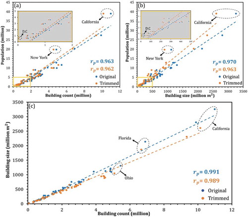
Figure 4. Performances of the four weighting scenarios in CONUS evaluated at the block group level. (a) building count; (b) building size; (c) building size*count; (d) uniform distribution in census tracts. Only trimmed building footprints are used in a-c

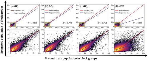
Figure 5. The 100 m population grid extracted using the $B{F}_s^{\prime }$ scenario.

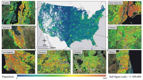
Figure 6. Scatter plot heatmap of the ground-truth population against the estimated population in block groups for 49 states (DC included) of the CONUS (dashed line represents regression line, and solid line represents the 1:1 reference line)

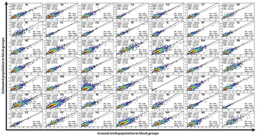
Figure 7. Six accuracy assessment metrics in the CONUS at the state level. RMSE (a); MAE (b); ORE (c); SE (d); CoE (e); and MIoA (f)

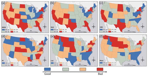
Table 5. Comparison of model performance between NYC and NY state. The metric values of the state and NYC (averaged in five counties) are highlighted in bold

Counties	# of BG*	RMSE	MAE	ORE	SE	COE	MIOA
NYC
Bronx	1,154	848.30	553.72	62.67%	37.95	−0.46	0.50
Kings	2,062	599.41	423.14	40.45%	22.18	−0.17	0.54
New York	1,167	1397.79	981.97	68.62%	138.05	−3.14	0.36
Queens	1,739	515.68	353.79	30.80%	5.17	0.36	0.64
Richmond	324	442.54	308.71	24.93%	−2.41	0.63	0.72
Averages above	/	760.74	524.27	45.49%	40.19	−0.55	0.55
NY State	15,405	599.18	345.71	31.81%	35.17	0.12	0.65

*BG represents the block group.

Table 6. Before and after building footprint trimming

Scenarios	RMSE	MAE	ORE	SE	CoE	MIoA
$B{F}_s$ (original)	462.40	316.27	27.74%	1.27	0.77	0.75
$B{F}_s^{\prime }$ (trimmed)	444.43	298.74	25.55%	3.51	0.79	0.76

Klein Goldewijk, K., Beusen, A., Van Drecht, G., & De Vos, M. (2011). The HYDE 3.1 spatially explicit database of human‐induced global land‐use change over the past 12,000 years. Global Ecology and Biogeography, 20(1), 73–86.

 Google Scholar

Doxsey-Whitfield, E., MacManus, K., Adamo, S. B., Pistolesi, L., Squires, J., Borkovska, O., & Baptista, S. R. (2015). Taking advantage of the improved availability of census data: A first look at the gridded population of the world, version 4. Papers in Applied Geography, 1(3), 226–234.

 Google Scholar

Balk, D., Deichmann, U., Yetman, G., Pozzi, F., Hay, S. I., & Nelson, A. (2006).  Determining global population distribution: Methods, applications and data. Advances in parasitology, 62, 119–156.

 Google Scholar

Freire, S., & Pesaresi, M. (2015). GHS population grid, derived from GPW4, multitemporal (1975, 1990, 2000, 2015). European Commission, Joint Research Centre (JRC). PID: http://data. europa.eu/89h/jrcghsl-ghs_pop_gpw4_globe_r2015a

 Google Scholar

Dobson, J. E., Bright, E. A., Coleman, P. R., Durfee, R. C., & Worley, B. A. (2000). LandScan: A global population database for estimating populations at risk. Photogrammetric Engineering and Remote Sensing, 66(7), 849–857.

 Google Scholar

Frye, C., Wright, D. J., Nordstrand, E., Terborgh, C., & Foust, J. (2018). Using classified and unclassified land cover data to estimate the footprint of human settlement. Data Science Journal, 17(20), 1–12.

 Google Scholar

Tatem, A. (2017). WorldPop, open data for spatial demography. Sci Data, 4(1), 2017.

 Google Scholar

Azar, D., Engstrom, R., Graesser, J., & Comenetz, J. (2013). Generation of fine-scale population layers using multi-resolution satellite imagery and geospatial data. Remote Sensing of Environment, 130, 219–232.

 Google Scholar

Tiecke, T. G., Liu, X., Zhang, A., Gros, A., Li, N., Yetman, G., … Dang, H. A. H. (2017). Mapping the world population one building at a time. arXiv, 1712, 05839.

 Google Scholar

Palacios-Lopez, D., Bachofer, F., Esch, T., & Heldens, W. (2019). New perspectives for mapping global population distribution using world settlement footprint products. Sustainability, 11(21), 6056.

 Google Scholar

Murdock, A. P., Harfoot, A. J. P., Martin, D., Cockings, S., & Hill, C. (2015). OpenPopGrid: An open gridded population dataset for England and Wales. GeoData, University of Southampton. http://openpopgrid.geodata.soton.ac.uk/

 Google Scholar

Data availability statement

The product can be visualized at http://arcg.is/19S4qK. To download the data, please visit https://doi.org/10.7910/DVN/DLGP7Y.