
Figures & data
Table 1. Selected use cases and their parameters
Figure 1. Location of our Amazonian target area marked on Google Maps (Google Maps, Citation2019)
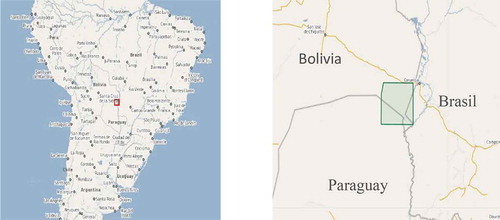
Figure 2. Location of our target area in Poland marked on Google Maps (Google Maps, Citation2019)
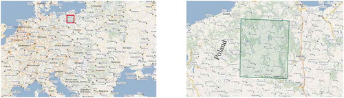
Figure 3. Location of our target area in Romania marked on Google Maps (Google Maps, Citation2019)
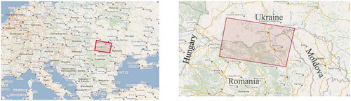
Figure 4. Location of our target area in Nebraska marked on Google Maps (Google Maps, Citation2019)
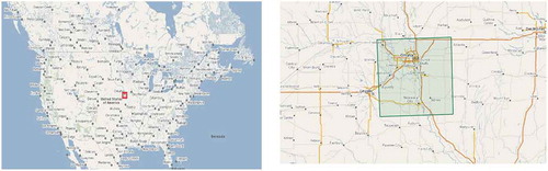
Figure 5. Our target area in Mozambique marked on Google Maps (Google Maps, Citation2019)
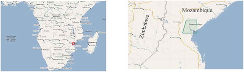
Figure 6. Locations of the selected cities marked on Google Maps (Google Maps, Citation2019)
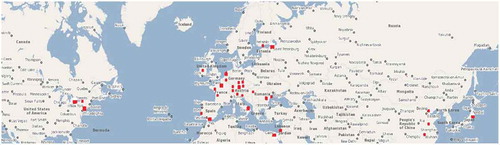
Figure 7. The View Model of CANDELA seen from three perspectives
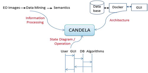
Figure 8. Block diagram of the CANDELA platform modules as information processing flow (Candela, Citation2019)
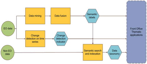
Figure 9. Architecture of the Data Mining module on the platform and front end (Datcu et al., Citation2019a)
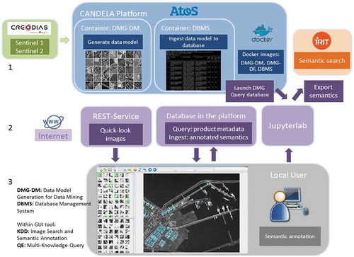
Figure 10. Data Mining functions, components, and interfaces
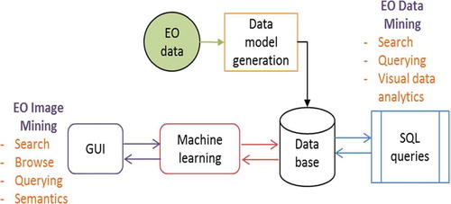
Figure 11. GUI interface of Image Mining (Top): Interactive interface to retrieve images belonging to the categories that exist in a collection (e.g., Smoke). The upper left half shows relevant retrieved patches, while the lower left half shows irrelevant retrieved patches. The large GUI panel on the right shows the image that is being worked on, and which can be zoomed. (Bottom): The same interactive interface, but in this case, the users can verify the selected training samples by checking their surroundings as there is a link between the patches in the upper left half and the right half. Here, the magenta color on the big quick-look panel shows the retrieved patches being similar to the ones provided by the user. The user can also see the selected patches selected by him/her as relevant and irrelevant patches (bottom part of the GUI)
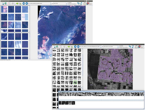
Table 2. Comparison between Shallow machine learning (ML), Deep Learning, and Active Learning
Figure 12. (a) Query interface of Data Mining. (Left:) Select the query parameters, e.g., “metadata_id”, “mission”, and “sensor” and enter the desired query values in the query-expression table below. (Right:) Display the products that match with the query criteria (“mission” = S2) including their metadata and image files. (b) Query interface of Data Mining. (Left:) Select the metadata parameters (e.g., “mission = S2A” and “metadata_id = 39”) and (Right) semantics parameters (e.g., “name = Smoke”). Depending on the EO user needs, it is possible to use only one or to combine these two queries. The combined query is returning the number of results from the database (in this case 543). (c) Query interface of Data Mining. This figure presents a list of images matching the query criteria (from Figure 12b). The upper part of the figure shows a table composed of several metadata columns corresponding to the patch information while the lower part of the figure presents a list of the quick-looks of patches that corresponds to the query
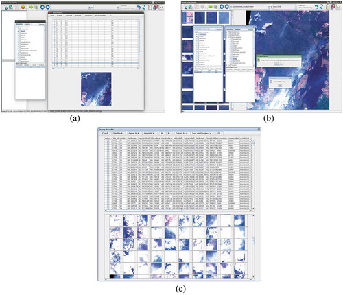
Figure 13. Operation state diagram of Data Mining
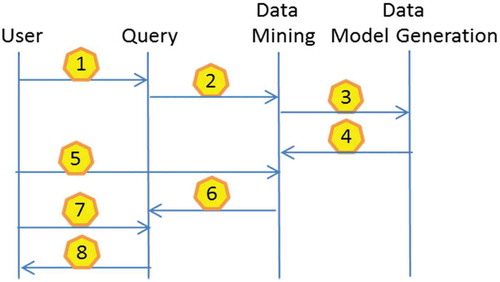
Table 3. The amount of data processed by the Data Mining module
Figure 14. A multi-temporal data set for the first use case. (From left to right and from top to bottom): Quick-look views of the first Sentinel-1 image from August 2nd, 2019, of the second image from August 26th, 2019, and of the last image from September 7th, 2019, followed by the classification map of each of the three images
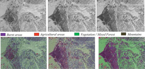
Figure 15. A multi-temporal data set for the first use case. (From left to right and from top to bottom): An RGB quick-look view of a first Sentinel-2 image from August 5th, 2019, of the second image from August 25th, 2019, and of the last image from September 9th, 2019, followed by the classification maps of each of the three images
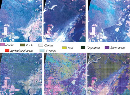
Figure 16. Diversity of categories, and the change of categories identified from three Sentinel-1 images (top) and three Sentinel-2 images (bottom) that cover the area of interest of the first use case. The Sentinel-1 images were acquired on August 2nd, 2019, August 26th, 2019, and on September 7th, 2019, while the Sentinel-2 images were acquired on August 5th, 2019, August 25th, 2019, and on September 9th, 2019
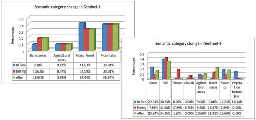
Figure 17. A multi-sensor and a multi-temporal data set for the second use case. (Top – from left to right): A quick-look view of a first Sentinel-2 image from July 30th, 2017, and its classification map, and a quick-look view of a second Sentinel-2 image from September 28th, 2017, and its classification map. (Bottom – from left to right): A quick-look view of a first Sentinel-1 image from July 30th, 2017, and its classification map, and a quick-look view of a second Sentinel-1 image from August 29th, 2017, and its classification map
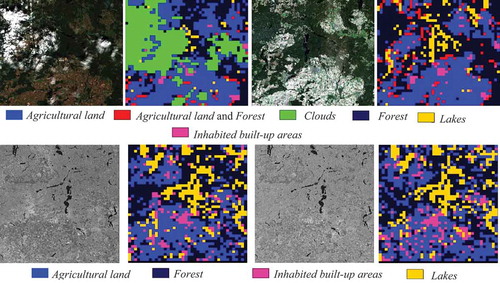
Figure 18. Diversity of categories identified from two Sentinel-2 and two Sentinel-1 images that cover the area of interest of the second use case. (From left to right and from top to bottom): The distribution of the retrieved and annotated categories of the Sentinel-2 images acquired on July 30th, 2017 and on September 28th, 2017, and the categories of the Sentinel-1 images acquired on July 30th, 2017 and on August 29th, 2017. The differences between the Sentinel-2 and Sentinel-1 results can be explained by clouds being only visible in Sentinel-2 images. For the different labels, see Section 4.2
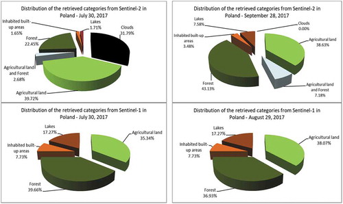
Figure 19. Semantic label changes between two Sentinel-1 images (right) and two Sentinel-2 images (left) acquired for the second use case. The value of the changes should be multiplied by 100 in order to obtain the percentage of the change. The results are given for the windstorms in Poland
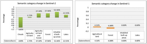
Figure 20. A multi-temporal data set for the fifth use case (From left to right, first two columns): A quick-look view of a first Sentinel-1 image from June 27th, 2015, and its classification map. (From left to right, last two columns): A quick-look view of a second Sentinel-1 image from September 1st, 2016, and its classification map
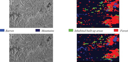
Figure 21. Diversity of categories identified from two Sentinel-1 images that cover the area of interest of the fifth use case. (From left to right): Distribution of the retrieved and annotated categories of the images acquired on June 27th, 2015, and on September 1st, 2016
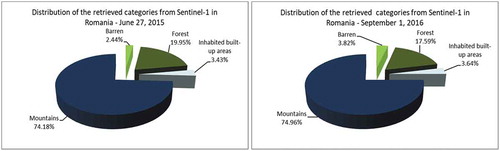
Figure 22. Semantic label changes between two Sentinel-1 images acquired for the fifth use case
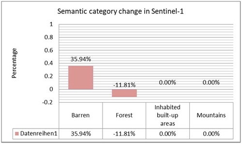
Figure 23. A multi-temporal data set for the third use case. (From left to right and from top to bottom): An RGB quick-look view of a first Sentinel-2 image from March 1st, 2018, of the second image from March 21st, 2018; and the last image from June 24th, 2018, followed by the classification maps of each of the three images
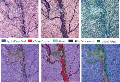
Figure 24. Distribution of retrieved semantic categories for the three images of the third use case, the floods in Omaha, Nebraska, USA
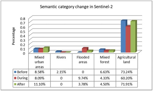
Figure 25. A multi-sensor data set for the fourth use case (Top -from left to right): A quick-look view of a Sentinel-1 image from March 19th, 2019, and its classification map. (Bottom -from left to right): An RGB quick-look view of a first Sentinel-2 image from March 22nd, 2019, and its classification map
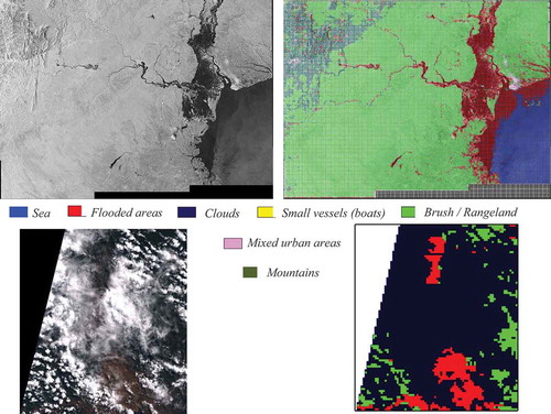
Figure 26. Diversity of categories identified from a Sentinel-1 image that covers the area of interest of the fourth use case
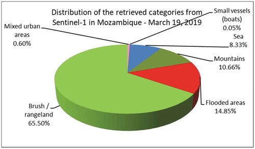
Figure 27. A multi-temporal data set for Tokyo and its surrounding areas. (Top -from left to right): A quick-look view of a first Sentinel-1 image from July 26th, 2019, and its classification map. (Bottom -from left to right): A quick-look view of a second Sentinel-2 image from May 8th, 2019, and its classification map
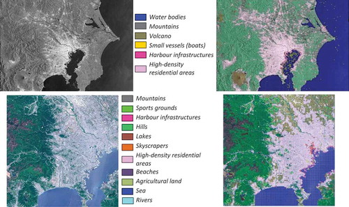
Figure 28. Diversity of categories extracted from a Sentinel-1 image and from a Sentinel-2 image that are covering the area of interest of Tokyo and its surrounding areas. (From left to right): The distribution of the retrieved and semantically annotated categories of the images acquired on July 26th, 2019, and on May 8th, 2019. The differences between Sentinel-1 and Sentinel-2 results are mainly due to the higher resolution of the Sentinel-2 data
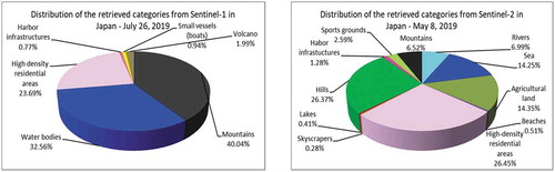
Figure 29. A multi-temporal data set for Amsterdam and its surrounding areas. (Top -from left to right): A quick-look view of a first Sentinel-1 image from March 22nd, 2016, and its classification map. (Bottom -from left to right): An RGB quick-look view of a second Sentinel-2 image from April 21st, 2016, and its classification map
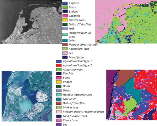
Figure 30. Diversity of categories identified from a Sentinel-1 image and from a Sentinel-2 image that are covering the area of interest of Amsterdam and its surrounding areas. (From left to right): The distribution of the retrieved and semantically annotated categories of the images acquired on March 22nd, 2016, and on April 21st, 2016. The differences between Sentinel-1 and Sentinel-2 results are mainly due to the higher resolution of the Sentinel-2 data
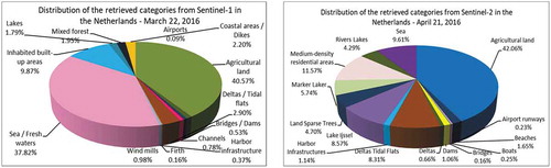
Figure 31. A data set for Saint Petersburg and its surrounding areas. (From left to right): An RGB quick-look view of a Sentinel-2 image from April 4th, 2019, and its classification map
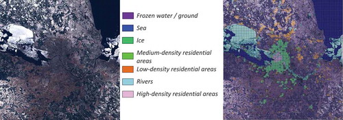
Figure 32. Diversity of categories identified from a Sentinel-2 image that is covering Saint Petersburg, Russia. This image was acquired on April 4th, 2019
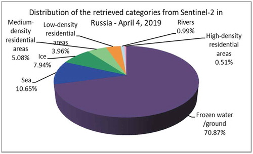
Figure 33. A data set for Cairo and its surrounding areas. (From left to right): An RGB quick-look view of a Sentinel-2 image from July 8th, 2019, and its classification map
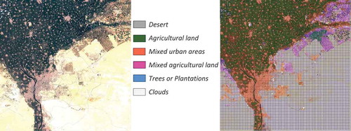
Figure 34. Diversity of categories identified from a Sentinel-2 image that is covering Cairo, Egypt. This image was acquired on July 8th, 2019
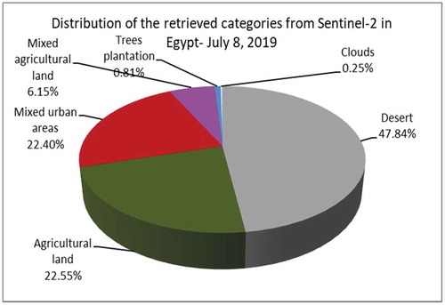
Figure 35. (a) Performance evaluation metrics for a selected number of man-made structures and natural categories retrieved from Sentinel-2 images. (b). Performance evaluation metrics for a selected number of man-made structures and natural categories retrieved from Sentinel-1
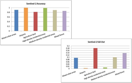
Figure 35. (Continued)
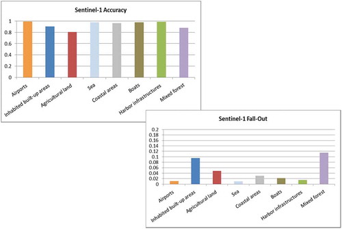
Figure 36. A data set of Aquila, Italy (acquired by the QuickBird sensor during an earthquake) and its surrounding areas. (From left to right): An RGB quick-look view of a QuickBird image from April 6th, 2009, and its classification map. The sensor parameters are described in QuickBird sensor parameter description and data access (QuickBird, Citation2020)
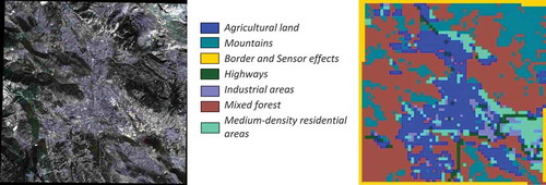
Figure 37. A data set of the French Riviera and its surrounding areas. (From left to right): An RGB quick-look view of a Spot-5 image from April 23rd, 2001, and its classification map. For classification three bands (band 1, 2, and 3) were selected. The sensor parameters are described in Spot sensor parameter description (Spot, Citation2020)
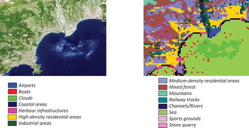
Figure 38. A data set of Venice, Italy and its surrounding areas. (From left to right): An RGB quick-look view of a WorldView-2 image from September 9th, 2012, and its classification map. From the available eight bands of the sensor we used for classification three bands (band 1, 2, and 3). The sensor parameters are described in WorldView sensor parameter description (WorldView, Citation2020)
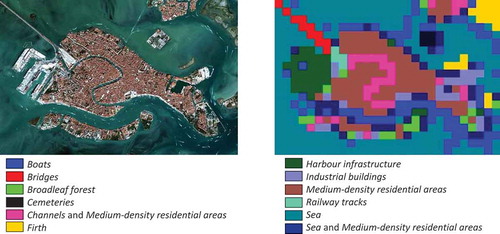
Figure 39. A data set of Calcutta, India (acquired by the Sentinel-3 sensor) and its surrounding areas. (From left to right): An RGB quick-look view of a Sentinel-3 image from January 8th, 2017, and its classification map. From the available 21 bands of the sensor we used for classification eight bands (band 1, 2, 3, 6, 12, 16, 19, and 21). The sensor parameters are described in Sentinel-3 sensor parameter description and data access (Sentinel-3, Citation2020)
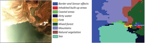
Figure 40. A data set of Amsterdam, the Netherlands and its surrounding areas. (From left to right): A quick-look view of a TerraSAR-X image from May 15th, 2015, and its classification map. The sensor parameters are described in TerraSAR-X sensor parameter description and data access (TerraSAR-X, Citation2020)
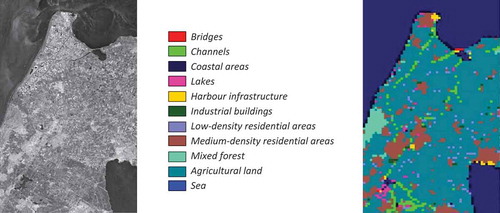
Figure 41. A data set of the Danube Delta, Romania and its surrounding areas. (From left to right): A quick-look view of a COSMO-SkyMed image from September 27th, 2007, and its classification map. The sensor parameters are described in COSMO-SkyMed (COSMO-SkyMed, Citation2020)
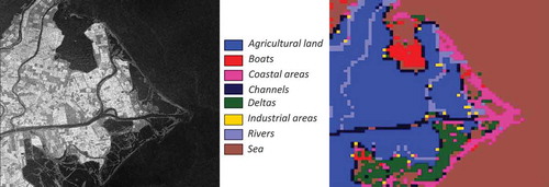
Figure 42. A data set of Vancouver, Canada and its surrounding areas. (From left to right): A quick-look view of a RADARSAT-2 image from April 16th, 2008, and its classification map. The sensor parameters are described in RADARSAT sensor parameter description (RADARSAT, Citation2020)
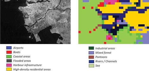
Figure 43. A data set of Berlin, Germany and its surrounding areas. (From left to right): A quick-look view of a Gaofen-3 image from July 27th, 2018, and its classification map. The sensor parameters are described in Gaofen-3 sensor parameter description (Gaofen-3, Citation2020)
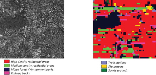
Table 4. Demonstration of the Big data achievements with the Data Mining module
Table 5. The achievements of the Data Mining module for each activity
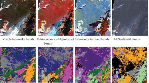
Figure 44. Visibility of different categories depending on the selection of the Sentinel-2 color bands. (From left to right, top): A quick-look view of visible false-color bands (B4, B3, and B2), false-colour visible/infrared bands (B8, B4, and B3), false-color infrared bands (B12, B11, and B8A), and all bands (B1, B2, B3, B4, B5, B6, B7, B8, B8A, B9, B10, B11, and B12). (From left to right, bottom): An example that shows four combination of bands and the information that can be extracted (Espinoza-Molina, Bahmanyar, Datcu, Díaz-Delgado, & Bustamante, Citation2017)
Data availability statement
For the moment, the data from the project are not publicly available. The data that support the findings of this study will be available on request from the authors.