Using open data to detect the structure and pattern of informal settlements: an outset to support inclusive SDGs’ achievement

Figures & data

Figure 1. Schematic comparison of Pixel-Based Classification (PBC) and Object-Based Classification (OBC). Top Row: on VHR, OBC more accurately detects vegetation, while PBC comprises mix pixels. Bottom Row: Spatial resolution and size of the pixels define either OBC or PBC can be more effective. Regarding MR, OBC is inefficient as a pixel contains more than one object, while PBC still detects vegetation (Source for the background satellite image: Google Earth Engine)

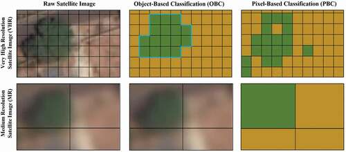
Figure 2. Random forest algorithm’s schematic function in image classification. The classifier consists of a collection of individual trees. Each tree independently offers a class prediction. The class with the most votes becomes the model prediction for image classification

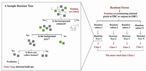
Figure 3. Study areas. Small rectangles numbered from 1–6 represent 2.4 km² sample areas for the visualisation and the magnification of the results

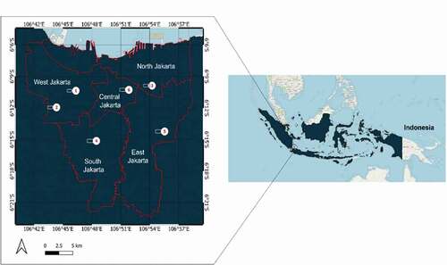
Figure 4. Informal settlements of Jakarta adapted from a map produced in 2015 (The World Bank 2015)

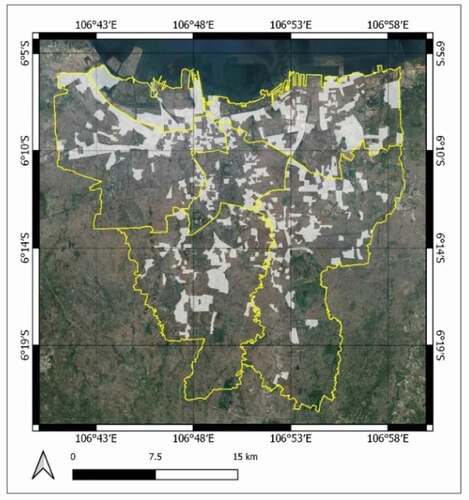
Figure 5. Overview of the procedure followed to detect informal settlements using medium resolution satellite images (MR), OpenStreetMap (OSM) and random forest machine learning algorithm (RF)

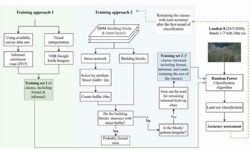
Table 1. Proposed classes for the classification of Landsat 8 in Jakarta

Training Classes	Description
Formal Build-up	Standard size building blocks with ample open space and vegetation in between.
Informal Build-up	Substandard housing with limited open space and vegetation in between.
Bare Soil	Undeveloped areas with no dominant vegetation cover.
Low Vegetation	Areas covered by low vegetation, such as grass.
Road	Street network and areas covered by asphalt.
High Vegetation	Areas dominated by trees.
Water	Areas covered by water, such as lakes, canals, and pools.
Cloud Mask	Areas of satellite image that are covered by cloud.

Figure 6. Left: Street structure in informal settlements in Jakarta. Numbers 1–4 represent the entry points to the informal settlements with no car accessibility (Source: Hidayati et al., 2020), Right: Urban fabric in informal settlements (Source: Alzamil, 2018)

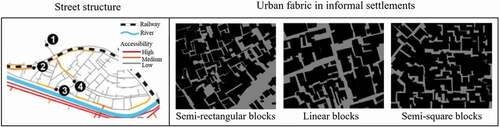
Figure 7. Using OpenStreetMap (OSM) for developing the training set for the informal built-up class. The blue areas represent the building with no access to a street or access to narrow streets that have been used to select pixels for informal settlements (Source for data layers: OpenStreetMap)

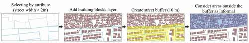
Table 2. Confusion Matrix of RF for the first round of classification. Least accuracy and precision relate to formal built-up in which mainly roads and informal built-up have been wrongly classified as formal

	Classes
Classes	Bare Soil	Formal Built-up	Low Vegetation	Informal Built-up	Roads	High Vegetation	Water	Cloud Mask	Precision	Accuracy
Bare Soil	75	5	9	0	3	0	2	1	0.76	0.93
Formal Built-up	1	60	2	16	9	4	0	3	0.58	0.88
Low Vegetation	9	2	76	0	2	1	5	0	0.75	0.93
Informal Built-up	6	14	4	62	8	1	0	0	0.72	0.91
Roads	1	14	0	7	59	5	8	1	0.60	0.88
High Vegetation	2	3	7	0	4	78	1	0	0.86	0.95
Water	0	3	2	1	9	2	77	1	0.81	0.94
Cloud Mask	4	3	1	0	4	0	2	81	0.93	0.97

Figure 8. First round of land-use and land cover classification on Landsat 8

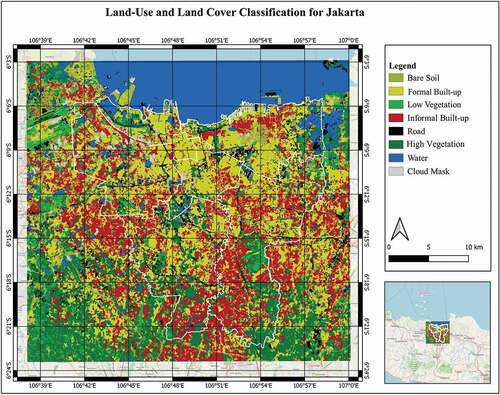
Figure 9. Second round of land-use and land cover classification on Landsat 8 using OSM for developing the training set

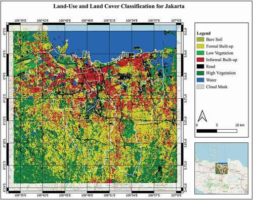
Figure 10. Informal (in red) and formal (in yellow) settlements detected in Jakarta. 1. Classification by RF machine learning algorithm through the traditional method of training. 2. Classification by RF which takes advantage of OSM for developing the training set

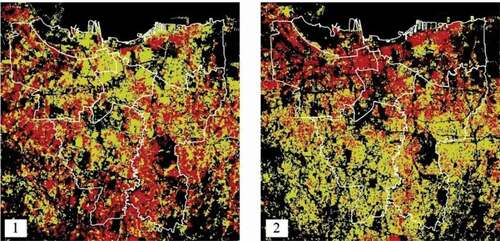
Table 3. Confusion Matrix of RF for the second round of classification

Classes
Classes	Bare Soil	Formal Built-up	Low Vegetation	Informal Built-up	Roads	High Vegetation	Water	Cloud Mask	Precision	Accuracy
Bare Soil	87	2	5	0	0	0	0	1	0.86	0.97
Formal Built-up	2	76	2	9	6	0	0	0	0.79	0.94
Low Vegetation	6	0	86	0	1	1	1	0	0.86	0.97
Informal Built-up	1	8	3	81	1	1	0	0	0.88	0.93
Roads	1	8	0	2	77	2	4	1	0.81	0.95
High Vegetation	1	1	4	0	3	85	1	0	0.93	0.98
Water	1	1	0	0	6	2	84	1	0.92	0.97
Cloud Mask	2	0	0	0	1	0	1	91	0.97	0.99

Figure 11. Comparison between the roads detected in the first and second round of classification (roads are mapped as black lines). Roads in the first round of classification are not continuous and represent some noise. Unlike the first-round results, street lines in the second round are mainly unbroken and demonstrate a high level of precision that is represented in Table 3

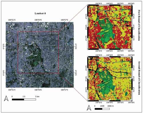
Figure 12. Sample areas (Nos. 1–6) for magnification of the informal settlement detection by RF

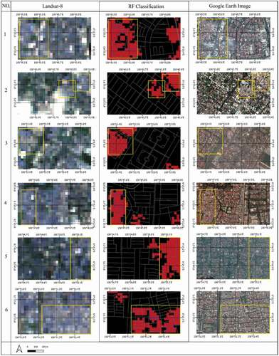
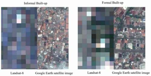
Figure 13. Colour composite of Landsat 8 pixels in formal vs. informal built-up

Bank, T. W. (2015). DKI Jakarta: Informal Settlement Mapping Jakarta. http://pubdocs.worldbank.org/en/408201444418421010/Output-DKI-JAKARTA-INFORMAL-SETTLEMENT-MAPPING.

 Google Scholar

Hidayati, I., Yamu, C., & Tan, W. (2020). Realised Pedestrian Accessibility of an Informal Settlement in Jakarta, Indonesia. Journal of Urbanism, 1–23. doi: https://doi.org/10.1080/17549175.2020.1814391.

 Google Scholar

Alzamil, W. S. (2018). Evaluating Urban Status of Informal Settlements in Indonesia: A Comparative Analysis of Three Case Studies in North Jakarta. Journal of Sustainable Development, 11(4), 148.

 Google Scholar

Data availability statement

Open data used for this study is freely available to public through the Copernicus Open Access Hub (https://scihub.copernicus.eu/) and OpenStreetMap Indonesia (https://openstreetmap.id/en/dki-jakarta/).