GIScience research challenges for realizing discrete global grid systems as a Digital Earth

Figures & data

Figure 1. Two methods of geographic object representation in the DGGS model. (a–c) Cell subset method and (d–e) Vertex cell subset. (a) point objects, (b) and (d) line objects, and (c) and (e) polygon objects.

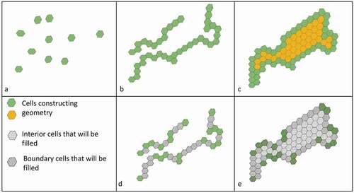
Table 1. Required metadata for different types of geographic model representations.

Method	Traditional model	DGGS-Based Model
Cell subset	Point	Only attributes
(Method 1)	Line	Attributes – order of cells
	Polygon	Attributes – order of cells – border cells – interior cells
	Raster Band	Value
Vertex cell subset
(Method 2)	Point	Only attributes
	Line	Order of cells
	Polygon	Order of cells
	Raster Band	Value

Figure 2. Overlap relation for two areal regions A and B in the traditional vector model.

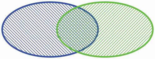
Figure 3. Overlap topological relation between two DGGS features $A$ and $B$ for the standard topological model.

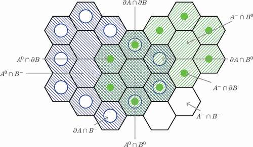
Figure 4. Overlap topological relation between two DGGS features $A$ and $B$ for Clementini and Di Felice’s topological relationship number 21 in their extended model (Clementini & Di Felice, 1996).

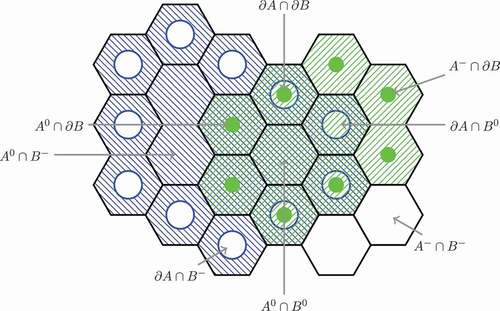
Figure 5. Temporal and geographical data integration for wildfire modelling. Each cube is representative of the specific theme for wildfire, and the cell size in each cube is representation of spatial resolution of the input data. The depth of each cube is the temporal dimension.

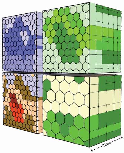
Figure 6. The decomposition of a sample rendering process on a server using current rendering engines (mapnik).

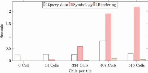
Figure 7. Two different buffer algorithm methods. (a) Using the cell subset method: (a1) A recursive method. In each iteration, we first find neighbours of the border cells of the object and add them as the new border, (a2) then add the previous border to the interior cell group and at the end, remove the common cells between the new border and new interior from the new border set of cells. (b) Using the vertex cell subset method: For each cell, in the border, we first find cells in the 6 main hexagonal directions that are at the buffer distance and then remove the duplicates and store them as a subset of cells.

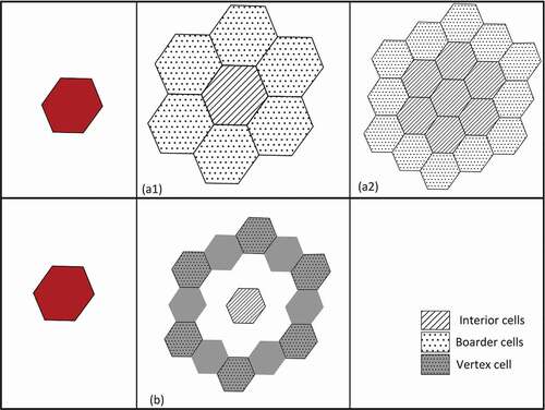
Figure 8. Intersection algorithm methods: (a) finding the intersection of two geometries using DGGID and the table join method and (b) finding intersecting objects with a minimum boundary hexagon and parent-child relations as auxiliary data.

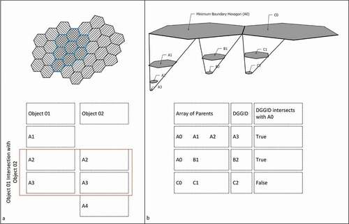
Table 2. A short summary of the current challenges for DGGS as a GIS and some of the existing research related to them.

Category	Research Challenge	Sample References
GIScience	Knowledge representation	2D data model: Tong et al. (2013); Robertson et al. (2020); Zhou, Chen, and Gong (2016)
		3D data model representation: Sirdeshmukh et al. (2019)
		Network topology: Dong, Chen, & Liu (2019)
	Scale	Uncertainty representation: Hojati et al. (2021, 2019); Li and Stefanakis (2020a)
		CA multi-scale analysis: Hojati and Robertson (2020)
		Convolution in a CNN context: Luo et al. (2019)
GISystems	Benchmarking	DGGS performance comparison: Robertson et al. (2020); Wang et al. (2021)
		Spatial operation comparison: Li and Stefanakis (2020b)
	Architecture	In database analytic: Robertson et al. (2020)
		Large-scale data storage: Li, McGrath, and Stefanakis (2021)
	Data I/O	Handling data sets: Mahdavi Amiri et al. (2019); Yang and Biuk-Aghai (2015); Tripathi et al. (2016)
		DGGS tiling and visualization: Mahdavi Amiri et al. (2019); Hall, Wecker, Ulmer, and Samavati (2020); Sherlock, Hasan, and Samavati (2021)

Clementini, E., & Di Felice, P. (1996). An algebraic model for spatial objects with indeterminate boundaries. London: CRC Press.

 Google Scholar

Tong, X. C., Ben, J., Liu, Y. Y., & Zhang, Y. S. (2013). Modeling and expression of vector data in the hexagonal discrete global grid system. In The international archives of the photogrammetry, remote sensing and spatial information sciences (Vol. XL-4-W2, pp. 15–25). Göttingen, Germany: Copernicus GmbH.

 Google Scholar

Robertson, C., Chiranjib, C., Majid, H., & Roberts, S. A. (2020). An integrated environmental analytics system (IDEAS) based on a DGGS. ISPRS Journal of Photogrammetry and Remote Sensing, 162, 214–228.

 Web of Science ®Google Scholar

Zhou, M., Chen, J., & Gong, J. (2016). A virtual globe-based vector data model: Quaternary quadrangle vector tile model. International Journal of Digital Earth, 9(3), 230–251.

 Web of Science ®Google Scholar

Sirdeshmukh, N., Verbree, E., Van Oosterom, P., Psomadaki, S., & Kodde, M. (2019). Utilizing a discrete global grid system for handling point clouds with varying locations, times, and levels of detail. Cartographica: The International Journal for Geographic Information and Geovisualization, 54(1), 4–15.

 Google Scholar

Dong, Q., Chen, J., & Liu, T. (2019). A topographically preserved road-network tile model and optimal routing method for virtual globes. Transactions in GIS, 23(2), 294–311.

 Web of Science ®Google Scholar

Hojati, M., Farmer, C., Feick, R., & Robertson, C. (2021). Decentralized geoprivacy: Leveraging social trust on the distributed web. International Journal of Geographical Information Science, 35(12), 2540–2566. doi: 10.1080/13658816.2021.1931236

 Web of Science ®Google Scholar

Hojati, M., Robertson, C., & Feick, R. (2019). Uncertainty-based representation of object-based spatial phenomena using discrete global grid systems data model. Presented at Global Water Futures Annual Science Meeting - GWF-2019, Saskatoon, SK, CA.

 Google Scholar

Li, M., & Stefanakis, E. (2020a). Geo-feature modeling uncertainties in discrete global grids: A case study of downtown Calgary, Canada. Geomatica, 74(4), 175–195.

 Google Scholar

Hojati, M., & Robertson, C. (2020). Integrating cellular automata and discrete global grid systems: A case study into wildfire modelling. AGILE: GIScience Series, 1, 6. Citation Key: agile-giss-1-6-2020.

 Google Scholar

Luo, J., Zhang, W., Su, J., & Xiang, F. (2019). Hexagonal convolutional neural networks for hexagonal grids. IEEE Access, Sorrento, Italy, 7, 142738–142749.

 Google Scholar

Wang, Z., Zhao, X., Sun, W., Luo, F., Yalu, L., & Duan, Y. (2021). Correlation analysis and reconstruction of the geometric evaluation indicator system of the discrete global grid. ISPRS International Journal of Geo-Information, 10(3), 115.

 Web of Science ®Google Scholar

Li, M., & Stefanakis, E. (2020b). Geospatial operations of discrete global grid systems—a comparison with traditional GIS. Journal of Geovisualization and Spatial Analysis, 4(2), 26.

 Google Scholar

Li, M., McGrath, H., & Stefanakis, E. (2021). Integration of heterogeneous terrain data into discrete global grid systems. Cartography and Geographic Information Science, 48(6), 1–19.

 Web of Science ®Google Scholar

Mahdavi Amiri, A., Alderson, T., & Samavati, F. (2019). Geospatial data organization methods with emphasis on aperture-3 hexagonal discrete global grid systems. Cartographica: The International Journal for Geographic Information and Geovisualization, 54(1), 30–50.

 Google Scholar

Yang, M., & Biuk-Aghai, R. (2015). Enhanced hexagon-tiling algorithm for map-like information visualisation VINCI ’15: Proceedings of the 8th International Symposium on Visual Information Communication and Interaction , Pages 137–142.

 Google Scholar

Tripathi, G., Sherlock, M. J., Amiri, A. M., & Samavati, F. (2016). Wavelet transforms for managing landsat data sets on a geospatial client-server discrete global grid system. In AGU Fall Meeting Abstracts, San Francisco, CA (Vol. 2016, pp. IN53B–1882).

 Google Scholar

Hall, J., Wecker, L., Ulmer, B., & Samavati, F. (2020). Disdyakis triacontahedron DGGS. ISPRS International Journal of Geo-Information, 9(5), 315.

 Web of Science ®Google Scholar

Sherlock, M. J., Hasan, M., & Samavati, F. F. (2021). Interactive data styling and multifocal visualization for a multigrid web-based Digital Earth. International Journal of Digital Earth, 14(3), 288–310.

 Web of Science ®Google Scholar

Data availability statement

Data used in this paper are available upon request from the corresponding author.