
Figures & data
Table 1. The Findable Accessible Interoperable and Reusable (FAIR) Guiding Principles for manual (human-driven) and automated (machine-driven) activities attempting to find and/or process scholarly/scientific digital data and non-data research objects – from data in the conventional sense to analytical pipelines (GO FAIR – International Support and Coordination Office, Citation2021; Wilkinson et al., Citation2016). Quoted from (Wilkinson et al., Citation2016), “four foundational principles – Findability, Accessibility, Interoperability, and Reusability (FAIR) – serve to guide [contemporary digital, e.g. web-based] producers and publishers” involved with “both manual [human-driven] and automated [machine-driven] activities attempting to find and process scholarly digital [data and non-data] research objects – from data [in the conventional sense] to analytical pipelines … An example of [scholarly/scientific digital] non-data research objects are analytical workflows, to be considered a critical component of the scholarly/scientific ecosystem, whose formal publication is necessary to achieve [transparency, scientific reproducibility and reusability]”. All scholarly/scientific digital data and non-data research objects, ranging from data in the conventional sense, either numerical or categorical variables as outcome (product), to analytical pipelines (processes), synonym for data and information processing systems, “benefit from application of these principles, since all components of the research process must be available to ensure transparency, [scientific] reproducibility and reusability”. Hence, “the FAIR principles apply not only to ‘data’ in the conventional sense, but also to the algorithms, tools, and workflows that led to that data … While there have been a number of recent, often domain-focused publications advocating for specific improvements in practices relating to data management and archival, FAIR differs in that it describes concise, domain-independent, high-level principles that can be applied to a wide range of scholarly [digital data and non-data] outputs. The elements of the FAIR Principles are related, but independent and separable. The Principles define characteristics that contemporary data resources, tools, vocabularies and infrastructures should exhibit to assist discovery and reuse by third-parties … Throughout the Principles, the phrase ‘(meta)data’ is used in cases where the Principle should be applied to both metadata and data.”
Figure 1. Group on Earth Observations (GEO)’s implementation plan for years 2005–2015 of the Global Earth Observation System of (component) Systems (GEOSS) (EC – European Commission and GEO – Group on Earth Observations, Citation2014; GEO – Group on Earth Observations, Citation2005, Citation2019; Mavridis, Citation2011), unaccomplished to date and revised by a GEO’s second implementation plan for years 2016–2025 of a new GEOSS, regarded as expert EO data-derived information and knowledge system (GEO – Group on Earth Observations, Citation2015; Nativi et al., Citation2015, Citation2020; Santoro et al., Citation2017). (a) Adapted from (EC – European Commission and GEO – Group on Earth Observations, Citation2014; Mavridis, Citation2011). Graphical representation of the visionary goal of the GEOSS applications. Nine “Societal Benefit Areas” are targeted by GEOSS: disasters, health, energy, climate, water, weather, ecosystems, agriculture and biodiversity. (b) Adapted from (EC – European Commission and GEO – Group on Earth Observations, Citation2014; Mavridis, Citation2011). GEO’s vision of a GEOSS, where interoperability of interconnected component systems is an open problem, to be accomplished in agreement with the Findable Accessible Interoperable and Reusable (FAIR) criteria for scientific data (product and process) management (GO FAIR – International Support and Coordination Office, Citation2021; Wilkinson et al., Citation2016), see . In the terminology of GEOSS, a digital Common Infrastructure is required to allow end-users to search for and access to the interconnected component systems. In practice, the GEOSS Common Infrastructure must rely upon a set of interoperability standards and best practices to interconnect, harmonize and integrate data, applications, models, and products of heterogeneous component systems (Nativi et al., Citation2015, p. 3). In 2014, GEO expressed the utmost recommendation that, for the next 10 years 2016–2025 (GEO – Group on Earth Observations, Citation2015), the second mandate of GEOSS is to evolve from an EO big data sharing infrastructure, intuitively referred to as data-centric approach (Nativi et al., Citation2020), to an expert EO data-derived information and knowledge system (Nativi et al., Citation2015, pp. 7, 22), intuitively referred to as knowledge-driven approach (Nativi et al., Citation2020). The formalization and use of the notion of Essential (Community) Variables and related instances (see ) contributes to the process of making GEOSS an expert information and knowledge system, capable of EO sensory data interpretation/transformation into Essential (Community) Variables in support of decision making (Nativi et al., Citation2015, p. 18, Citation2020). By focusing on the delivery to end-users of EO sensory data-derived Essential (Community) Variables as information sets relevant for decision-making, in place of delivering low-level EO big sensory data, the Big Data requirements of the GEOSS digital Common Infrastructure are expected to decrease (Nativi et al., Citation2015, p. 21, Citation2020).
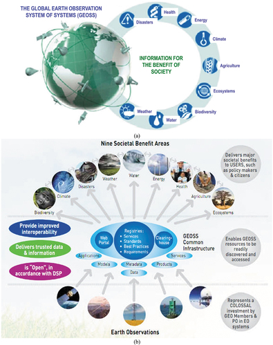
Table 2. Essential climate variables (ECVs) defined by the World Climate Organization (WCO) (Bojinski et al., Citation2014), pursued by the European Space Agency (ESA) Climate Change Initiative’s parallel projects (ESA – European Space Agency, Citation2017b, Citation2020a, Citation2020b) and by the Group on Earth Observations (GEO)’s second implementation plan for years 2016–2025 of the Global Earth Observation System of (component) Systems (GEOSS) (GEO – Group on Earth Observations, Citation2015; Nativi et al., Citation2015, Citation2020; Santoro et al., Citation2017), see . In the terrestrial layer, ECVs are: River discharge, water use, groundwater, lakes, snow cover, glaciers and ice caps, ice sheets, permafrost, albedo, land cover (including vegetation types), fraction of absorbed photosynthetically active radiation, leaf area index (LAI), above-ground biomass, soil carbon, fire disturbance, soil moisture. All these ECVs can be estimated from Earth observation (EO) imagery by means of either physical or semi-empirical data models, e.g. Clever’s semi-empirical model for pixel-based LAI estimation from multi-spectral (MS) imagery (Van der Meer & De Jong, Citation2011).
Figure 2. Two examples of semantic/ontological interoperability over heterogeneous sensory data sources (true-facts, observables). The first example is provided by the demonstrator of the Satellite Image Automatic Mapper™ (SIAM™) lightweight computer program (Baraldi, Citation2017, Citation2019a; Baraldi et al., Citation2010a, Citation2010b, Citation2018a, Citation2018b; Baraldi, Puzzolo, Blonda, Bruzzone, & Tarantino, Citation2006; Baraldi & Tiede, Citation2018a, Citation2018b), installed onto the Serco ONDA Data and Information Access Services (DIAS) Marketplace (Baraldi, Citation2019a). This demonstrator works as proof-of-concept of an Artificial General Intelligence (AGI) (Bills, Citation2020; Chollet, Citation2019; Dreyfus, Citation1965, Citation1991, Citation1992; EC – European Commission, Citation2019; Fjelland, Citation2020; Hassabis et al., Citation2017; Ideami, Citation2021; Jajal, Citation2018; Jordan, Citation2018; Mindfire Foundation, Citation2018; Mitchell, Citation2021; Practical AI, Citation2020; Saba, Citation2020c; Santoro et al., Citation2021; Sweeney, Citation2018a; Thompson, Citation2018; Wolski, Citation2020a, Citation2020b), suitable for Earth observation (AGI4EO) applications, namely, ‘AGI for Data and Information Access Services (DIAS) = AGI4DIAS = AGI-enabled DIAS = Semantics-enabled DIAS 2.0 (DIAS 2nd generation) = AGI + DIAS 1.0 + Semantic content-based image retrieval (SCBIR) + Semantics-enabled information/knowledge discovery (SEIKD)’ = EquationEquation (1)(1)
(1) , envisioned by portions of the existing literature (Augustin, Sudmanns, Tiede, & Baraldi, Citation2018; Augustin, Sudmanns, Tiede, Lang, & Baraldi, Citation2019; Baraldi, Citation2017; Baraldi & Tiede, Citation2018a, Citation2018b; Baraldi, Tiede, Sudmanns, Belgiu, & Lang, Citation2016; Baraldi, Tiede, Sudmanns, & Lang, Citation2017; Dhurba & King, Citation2005; FFG – Austrian Research Promotion Agency, Citation2015, Citation2016, Citation2018, Citation2020; Planet, Citation2018; Smeulders, Worring, Santini, Gupta, & Jain, Citation2000; Sudmanns, Augustin, van der Meer, Baraldi, and Tiede, Citation2021; Sudmanns, Tiede, Lang, & Baraldi, Citation2018; Tiede, Baraldi, Sudmanns, Belgiu, & Lang, Citation2017). In the present work, an integrated AGI4DIAS infrastructure = ‘AGI + DIAS 1.0 + SCBIR + SEIKD = DIAS 2.0ʹ is proposed as viable alternative to, first, traditional metadata text-based image retrieval systems, such as popular EO (raster-based) data cubes (Open Data Cube, Citation2020; Baumann, Citation2017; CEOS – Committee on Earth Observation Satellites, Citation2020; Giuliani et al., Citation2017, Citation2020; Lewis et al., Citation2017; Strobl et al., Citation2017), including the European Commission (EC) DIAS 1st generation (DIAS 1.0) (EU – European Union, Citation2017, Citation2018), and, second, prototypical content-based image retrieval (CBIR) systems, whose queries are input with text information, summary statistics or by either image, object or multi-object examples (Datta, Joshi, Li, & Wang, Citation2008; Kumar, Berg, Belhumeur, & Nayar, Citation2011; Ma & Manjunath, Citation1997; Shyu et al., Citation2007; Smeulders et al., Citation2000; Smith & Chang, Citation1996; Tyagi, Citation2017). Typically, existing DIAS and prototypical CBIR systems are affected by the so-called data-rich information-poor (DRIP) syndrome (Ball, Citation2021; Bernus & Noran, Citation2017). Figure captions are as follows. (a) Mosaic of twenty-nine 12-band Sentinel-2 images, acquired across Europe on 19 April, 2019, radiometrically calibrated into top-of-atmosphere reflectance (TOARF) values, depicted in true-colors, 10 m resolution, equivalent to a QuickLook™ technology. (b) Mosaic of three 11-band Landsat-8 images acquired across Europe on 21 April, 2019, radiometrically calibrated into TOARF values, depicted in true-colors, 30 m resolution, equivalent to a QuickLook technology. (c) Overlap between two SIAM’s output maps in semi-symbolic color names (Baraldi, Citation2017, Citation2019a; Baraldi et al., Citation2010a, Citation2010b, Citation2018a, Citation2018b, Citation2006; Baraldi & Tiede, Citation2018a, Citation2018b), automatically generated in near real-time from, respectively, the input 10 m resolution Sentinel-2 image mosaic, shown in Figure 2(a), and the 30 m resolution Landsat-8 image mosaic shown in Figure 2(b). The same map legend applies to the two input data sets. Semantic (symbolic) interoperability is accomplished by SIAM, independent of the input data source. In practice, SIAM instantiates a QuickMap™ technology, where a categorical map, provided with its discrete and finite map legend, is sensory data-derived automatically, without human-machine interaction and in near real-time, either on-line or off-line. (d) Zoom-in of the two SIAM maps, featuring the same semantics, independent of changes in the input sensory data source. In practice, SIAM accomplishes semantic interoperability by featuring robustness to changes in input data and scalability to changes in sensor specifications. (e) Second example of semantic interoperability over heterogeneous sensory data sources. Taken from Google Earth = Google Maps_Satellite View, it is equivalent to a QuickLook technology. It shows multi-source sensory data (quantitative/unequivocal information-as-thing) (Baraldi & Tiede, Citation2018a, Citation2018b; Capurro & Hjørland, Citation2003), equivalent to subsymbolic numerical variables, to be interpreted by users. (f) Taken from Google Maps_Map View (qualitative/equivocal information-as-data-interpretation) (Baraldi & Tiede, Citation2018a, Citation2018b; Capurro & Hjørland, Citation2003), equivalent to a symbolic interpretation of Google Maps_Satellite View data. In practice, Google Maps_Map View works as QuickMap technology. To be run automatically and in near real-time, either on-line or off-line, a QuickMap technology accomplishes data compression through discretization/categorization, together with interpretation of a continuous or discrete numerical variable belonging to a (2D) image-plane into a discrete and finite categorical variable provided with semantics, belonging to an ontology (mental model, conceptual model) of the 4D geospace-time real-world (Baraldi, Citation2017; Baraldi & Tiede, Citation2018a, Citation2018b; Matsuyama & Hwang, Citation1990).
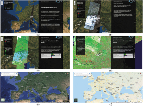
Figure 3. Adapted from (Ahlqvist, Citation2008; Di Gregorio, Citation2016; Di Gregorio & Jansen, Citation2000; Owers et al., Citation2021). Example of a standard land cover (LC) class taxonomy, developed by the geographic information science (GIScience) community (Buyong, Citation2007; Couclelis, Citation2010, Citation2012; Ferreira et al., Citation2014; Fonseca et al., Citation2002; Goodchild et al., Citation2007; Hitzler et al., Citation2012; Kuhn, Citation2005; Longley et al., Citation2005; Maciel et al., Citation2018; Sheth, Citation2015; Sonka et al., Citation1994; Stock et al., Citation2011; Hu, Citation2017). In conceptual terms, a taxonomy (legend) of LC classes is a hierarchical (multi-level, featuring inter-level parent-child relationships) vocabulary of entities (referents, classes of real-world objects) (Ball, Citation2021; Chen, Citation1976). Any LC class taxonomy is part-of a conceptual world model (world ontology, mental model of the world) (Baraldi, Citation2017; Baraldi & Tiede, Citation2018a, Citation2018b; Matsuyama & Hwang, Citation1990), consisting of entities (Ball, Citation2021; Chen, Citation1976), inter-entity relationships/predicates (Ball, Citation2021; Chen, Citation1976), facts (Campagnola, Citation2020), events/occurrents and processes/phenomena (Ferreira et al., Citation2014; Fonseca et al., Citation2002; Galton & Mizoguchi, Citation2009; Kuhn, Citation2005; Maciel et al., Citation2018; Tiede et al., Citation2017). Proposed by the Food and Agriculture Organization (FAO) of the United Nations (UN), the well-known hierarchical Land Cover Classification System (LCCS) taxonomy (Di Gregorio & Jansen, Citation2000) is two-stage and fully-nested. It consists of a first-stage fully-nested 3-level 8-class FAO LCCS Dichotomous Phase (DP) taxonomy, which is general-purpose, user- and application-independent. It consists of a sorted set of three dichotomous layers (Di Gregorio & Jansen, Citation2000): (i) Primarily Vegetated versus Primarily Non-Vegetated. In more detail, Primarily Vegetated applies to areas whose vegetative cover is at least 4% for at least two months of the year. Vice versa, Primarily Non-Vegetated areas have a total vegetative cover of less than 4% for more than 10 months of the year. (ii) Terrestrial versus aquatic. (iii) Managed versus natural or semi-natural. These three dichotomous layers deliver as output the following 8-class FAO LCCS-DP taxonomy. (A11) Cultivated and Managed Terrestrial (non-aquatic) Vegetated Areas. (A12) Natural and Semi-Natural Terrestrial Vegetation. (A23) Cultivated Aquatic or Regularly Flooded Vegetated Areas. (A24) Natural and Semi-Natural Aquatic or Regularly Flooded Vegetation. (B35) Artificial Surfaces and Associated Areas. (B36) Bare Areas. (B47) Artificial Waterbodies, Snow and Ice. (B48) Natural Waterbodies, Snow and Ice. The general-purpose user- and application-independent 3-level 8-class FAO LCCS-DP taxonomy is preliminary to a second-stage FAO LCCS Modular Hierarchical Phase (MHP) taxonomy, consisting of a battery of user- and application-specific one-class classifiers, equivalent to one-class grammars (syntactic classifiers) (Di Gregorio & Jansen, Citation2000). In recent years, the two-phase FAO LCCS taxonomy has become increasingly popular (Ahlqvist, Citation2008; Durbha et al., Citation2008; Herold et al., Citation2009, Citation2006; Jansen et al., Citation2008; Owers et al., Citation2021). For example, it is adopted by the ongoing European Space Agency (ESA) Climate Change Initiative’s parallel projects (ESA – European Space Agency, Citation2017b, Citation2020a, Citation2020b). One reason for its popularity is that the FAO LCCS hierarchy is “fully nested” while alternative LC class hierarchies, such as the Coordination of Information on the Environment (CORINE) Land Cover (CLC) taxonomy (Bossard et al., Citation2000), the U.S. Geological Survey (USGS) Land Cover Land Use (LCLU) taxonomy by J. Anderson (Lillesand & Kiefer, Citation1979), the International Global Biosphere Programme (IGBP) DISCover Data Set Land Cover Classification System (EC – European Commission, Citation1996) and the EO Image Librarian LC class legend (Dumitru et al., Citation2015), start from a first-level taxonomy which is already multi-class.
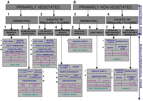
Figure 4. Adapted from (Tyagi, Citation2017). Typical architecture of a content-based image retrieval (CBIR) system (Datta et al., Citation2008; Kumar et al., Citation2011; Ma & Manjunath, Citation1997; Shyu et al., Citation2007; Smeulders et al., Citation2000; Smith & Chang, Citation1996; Tyagi, Citation2017), whose prototypical instantiations have been presented in the remote sensing (RS) and computer vision (CV) literature as an alternative to traditional metadata text-based image retrieval systems in operational mode (Airbus, Citation2018; Planet, Citation2017). CBIR system prototypes support no semantic CBIR (SCBIR) operation because they lack ‘Computer Vision (CV) ⊃ EO image understanding (EO-IU)’ capabilities, i.e. they lack “intelligence” required to transform EO big sensory data into systematic, operational, timely and comprehensive information-as-data-interpretation (Capurro & Hjørland, Citation2003), known that relationship ‘EO-IU ⊂ CV ⊂ Artificial General Intelligence (AGI) ⊂ Cognitive science’ = EquationEquation (2)(2)
(2) holds (Bills, Citation2020; Chollet, Citation2019; Dreyfus, Citation1965, Citation1991, Citation1992; EC – European Commission, Citation2019; Fjelland, Citation2020; Hassabis et al., Citation2017; Ideami, Citation2021; Jajal, Citation2018; Jordan, Citation2018; Mindfire Foundation, Citation2018; Mitchell, Citation2021; Practical AI, Citation2020; Saba, Citation2020c; Santoro et al., Citation2021; Sweeney, Citation2018a; Thompson, Citation2018; Wolski, Citation2020a, Citation2020b).
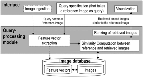
Figure 5. Cloud classification according to the U.S. National Weather Service (U.S. National Weather Service, Citation2019). “Ice clouds, also called cirrus clouds, which include cirrus, cirrostratus, and cirrocumulus, are made up of ice crystals” (Borduas & Donahue, Citation2018). Located in the upper troposphere (6–10 km) or lower stratosphere (10–16 km) (Borduas & Donahue, Citation2018; NIWA – National Institute of Water and Atmospheric Research, Citation2018; U.S. National Weather Service, Citation2019; UCAR – University Corporation for Atmospheric Research, Center for Science Education – SCIED, Citation2018). Worth mentioning, the troposphere is typically located between 0 and 10 km of height (Borduas & Donahue, Citation2018; NIWA – National Institute of Water and Atmospheric Research, Citation2018; U.S. National Weather Service, Citation2019; UCAR – University Corporation for Atmospheric Research, Center for Science Education – SCIED, Citation2018), known that the height of the top of the troposphere, called the tropopause (NIWA – National Institute of Water and Atmospheric Research, Citation2018), varies with latitude (it is lowest over the Poles and highest at the equator) and by season (it is lower in winter and higher in summer) (UCAR – University Corporation for Atmospheric Research, Center for Science Education – SCIED, Citation2018). In more detail, the tropopause can be as high as 20 km near the equator and as low as 7 km over the Poles in winter (NIWA – National Institute of Water and Atmospheric Research, Citation2018; UCAR – University Corporation for Atmospheric Research, Center for Science Education – SCIED, Citation2018). Given that, above the troposphere, the stratosphere is typically located between 10 and 30 km of height (Baraldi, Citation2017; Borduas & Donahue, Citation2018; NIWA – National Institute of Water and Atmospheric Research, Citation2018; U.S. National Weather Service, Citation2019; UCAR – University Corporation for Atmospheric Research, Center for Science Education – SCIED, Citation2018).
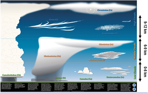
Figure 6. Adapted from (Baraldi & Tiede, Citation2018a, Citation2018b). Physical model, known a priori (available in addition to data), of the Sun-cloud-satellite geometry for arbitrary viewing and illumination conditions. Left: Actual 3D representation of the Sun/ cloud/ cloud–shadow geometry. Cloud height, h, is a typical unknown variable. Right: Apparent Sun/ cloud/ cloud–shadow geometry in a 2D soil projection, with ag = h ⋅ tanφβ, bg = h ⋅ tanφμ.
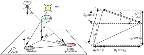
Figure 7. Adapted from (Swain & Davis, Citation1978). In the y-axis, reflectance values in physical range [0.0, 1.0] are represented as % values in range [0.0, 100.0], either ‘Top-of-atmosphere reflectance (TOARF) ⊇ Surface reflectance (SURF) ⊇ Surface albedo’ = EquationEquation (8)(8)
(8) (refer to the farther Subsection 3.3.2), where surface albedo is included in the list of terrestrial Essential Climate Variables (ECVs) defined by the World Climate Organization (WCO), see . This graph shows the typical spectral response characteristics of “green (photosynthetically active) vegetation” in reflectance values (Liang, Citation2004; Swain & Davis, Citation1978), where chlorophyll absorption phenomena occur jointly with water content absorption phenomena, according to a convergence-of-evidence approach (Baraldi, Citation2017; Baraldi & Tiede, Citation2018a, Citation2018b; Matsuyama & Hwang, Citation1990). “In general, the total reflectance of a given object across the entire solar spectrum (also termed albedo) is strongly related to the physical condition of the relevant targets (shadowing effects, slope and aspect, particle size distribution, refraction index, etc.), whereas the spectral peaks or, vice versa, absorption valleys are more closely related to the chemical condition of the sensed target (material surface-specific absorption)” (Van der Meer & De Jong, Citation2011, p. 251). In the remote sensing (RS) literature and in the RS meta-science common practice, chlorophyll absorption phenomena are traditionally intercepted by so-called vegetation spectral indexes, such as the well-known two-band Normalized Difference Vegetation Index, NDVI (DLR – Deutsches Zentrum für Luft-und Raumfahrt e.V. and VEGA Technologies, Citation2011; ESA – European Space Agency, Citation2015; Jordan, Citation1969; Liang, Citation2004; Neduni & Sivakumar, Citation2019; Rouse, Haas, Scheel, & Deering, Citation1974; Sykas, Citation2020; Tucker, Citation1979), where NDVI ∈ [−1.0, 1.0] = f1(Red, NIR) = f1(Red0.65÷0.68, NIR0.78÷0.90) = (NIR0.78÷0.90 – Red0.65÷0.68)/(NIR0.78÷0.90 + Red0.65÷0.68), which is monotonically increasing with the dimensionless Vegetation Ratio Index (VRI), where VRI ∈ (0, +∞) = NIR0.78÷0.90/Red0.65÷0.68 = (1. + NDVI)/(1. – NDVI) (Liang, Citation2004). Water content absorption phenomena in phenology are traditionally intercepted by so-called moisture or, vice versa, drought spectral indexes, such as the two-band Normalized Difference Moisture Index, NDMI (Liang, Citation2004; Neduni & Sivakumar, Citation2019; Sykas, Citation2020), equivalent to the Normalized Difference Water Index defined by Gao, NDWIGao (Gao, Citation1996), where NDMI ∈ [−1.0, 1.0] = NDWIGao = f2(NIR, MIR1) = f2(NIR0.78÷0.90, MIR1.57÷1.65) = (NIR0.78÷0.90 – MIR1.57÷1.65)/(NIR0.78÷0.90 + MIR1.57÷1.65), which is inversely related to the so-called Normalized Difference Bare Soil Index (NDBSI), NDBSI ∈ [−1.0, 1.0] = f3(NIR, MIR1) = (MIR1.55÷1.75 – NIR0.78÷0.90)/(MIR1.55÷1.75 + NIR0.78÷0.90) adopted in (Kang Lee, Dev Acharya, & Ha Lee, Citation2018; Roy, Miyatake, & Rikimaru, Citation2009), see . Popular two-band spectral indexes are conceptually equivalent to the angular coefficient/ slope/ 1st-order derivative of a tangent to the spectral signature in one point (Baraldi, Citation2017, Citation2019a; Baraldi et al., Citation2010a, Citation2010b, Citation2018a, Citation2018b, Citation2006; Baraldi & Tiede, Citation2018a, Citation2018b; Liang, Citation2004). Three-band spectral indexes are conceptually equivalent to a 2nd-order derivative as local measure of function concavity (Baraldi, Citation2017, Citation2019a; Baraldi et al., Citation2010a, Citation2010b, Citation2018a, Citation2018b, Citation2006; Baraldi & Tiede, Citation2018a, Citation2018b; Liang, Citation2004). Noteworthy, no combination of derivatives of any order can work as set of basis functions, capable of universal function approximation (Bishop, Citation1995; Cherkassky & Mulier, Citation1998). It means that if, in the fundamental feature engineering phase (Koehrsen, Citation2018) preliminary to feature (pattern) recognition (analysis, classification, understanding), any two-band or three-band scalar spectral index extraction occurs, then it always causes an irreversible loss in (lossy compression of) the multivariate shape and multivariate intensity information components of a spectral signature (Baraldi, Citation2017, Citation2019a; Baraldi et al., Citation2010a, Citation2010b, Citation2018a, Citation2018b, Citation2006; Baraldi & Tiede, Citation2018a, Citation2018b).
![Figure 7. Adapted from (Swain & Davis, Citation1978). In the y-axis, reflectance values in physical range [0.0, 1.0] are represented as % values in range [0.0, 100.0], either ‘Top-of-atmosphere reflectance (TOARF) ⊇ Surface reflectance (SURF) ⊇ Surface albedo’ = EquationEquation (8)(8) \lsquoDNs≥ 0atEOLevel0⊇TOARF∈0.0, 1.0atEOLevel1⊇SURF∈0.0, 1.0atEOLevel2/currentARD⊇Surfacealbedo∈0.0, 1.0at,say,EOLevel3/nextgenerationARD\rsquo(8)(8) (refer to the farther Subsection 3.3.2), where surface albedo is included in the list of terrestrial Essential Climate Variables (ECVs) defined by the World Climate Organization (WCO), see Table 2. This graph shows the typical spectral response characteristics of “green (photosynthetically active) vegetation” in reflectance values (Liang, Citation2004; Swain & Davis, Citation1978), where chlorophyll absorption phenomena occur jointly with water content absorption phenomena, according to a convergence-of-evidence approach (Baraldi, Citation2017; Baraldi & Tiede, Citation2018a, Citation2018b; Matsuyama & Hwang, Citation1990). “In general, the total reflectance of a given object across the entire solar spectrum (also termed albedo) is strongly related to the physical condition of the relevant targets (shadowing effects, slope and aspect, particle size distribution, refraction index, etc.), whereas the spectral peaks or, vice versa, absorption valleys are more closely related to the chemical condition of the sensed target (material surface-specific absorption)” (Van der Meer & De Jong, Citation2011, p. 251). In the remote sensing (RS) literature and in the RS meta-science common practice, chlorophyll absorption phenomena are traditionally intercepted by so-called vegetation spectral indexes, such as the well-known two-band Normalized Difference Vegetation Index, NDVI (DLR – Deutsches Zentrum für Luft-und Raumfahrt e.V. and VEGA Technologies, Citation2011; ESA – European Space Agency, Citation2015; Jordan, Citation1969; Liang, Citation2004; Neduni & Sivakumar, Citation2019; Rouse, Haas, Scheel, & Deering, Citation1974; Sykas, Citation2020; Tucker, Citation1979), where NDVI ∈ [−1.0, 1.0] = f1(Red, NIR) = f1(Red0.65÷0.68, NIR0.78÷0.90) = (NIR0.78÷0.90 – Red0.65÷0.68)/(NIR0.78÷0.90 + Red0.65÷0.68), which is monotonically increasing with the dimensionless Vegetation Ratio Index (VRI), where VRI ∈ (0, +∞) = NIR0.78÷0.90/Red0.65÷0.68 = (1. + NDVI)/(1. – NDVI) (Liang, Citation2004). Water content absorption phenomena in phenology are traditionally intercepted by so-called moisture or, vice versa, drought spectral indexes, such as the two-band Normalized Difference Moisture Index, NDMI (Liang, Citation2004; Neduni & Sivakumar, Citation2019; Sykas, Citation2020), equivalent to the Normalized Difference Water Index defined by Gao, NDWIGao (Gao, Citation1996), where NDMI ∈ [−1.0, 1.0] = NDWIGao = f2(NIR, MIR1) = f2(NIR0.78÷0.90, MIR1.57÷1.65) = (NIR0.78÷0.90 – MIR1.57÷1.65)/(NIR0.78÷0.90 + MIR1.57÷1.65), which is inversely related to the so-called Normalized Difference Bare Soil Index (NDBSI), NDBSI ∈ [−1.0, 1.0] = f3(NIR, MIR1) = (MIR1.55÷1.75 – NIR0.78÷0.90)/(MIR1.55÷1.75 + NIR0.78÷0.90) adopted in (Kang Lee, Dev Acharya, & Ha Lee, Citation2018; Roy, Miyatake, & Rikimaru, Citation2009), see Table 3. Popular two-band spectral indexes are conceptually equivalent to the angular coefficient/ slope/ 1st-order derivative of a tangent to the spectral signature in one point (Baraldi, Citation2017, Citation2019a; Baraldi et al., Citation2010a, Citation2010b, Citation2018a, Citation2018b, Citation2006; Baraldi & Tiede, Citation2018a, Citation2018b; Liang, Citation2004). Three-band spectral indexes are conceptually equivalent to a 2nd-order derivative as local measure of function concavity (Baraldi, Citation2017, Citation2019a; Baraldi et al., Citation2010a, Citation2010b, Citation2018a, Citation2018b, Citation2006; Baraldi & Tiede, Citation2018a, Citation2018b; Liang, Citation2004). Noteworthy, no combination of derivatives of any order can work as set of basis functions, capable of universal function approximation (Bishop, Citation1995; Cherkassky & Mulier, Citation1998). It means that if, in the fundamental feature engineering phase (Koehrsen, Citation2018) preliminary to feature (pattern) recognition (analysis, classification, understanding), any two-band or three-band scalar spectral index extraction occurs, then it always causes an irreversible loss in (lossy compression of) the multivariate shape and multivariate intensity information components of a spectral signature (Baraldi, Citation2017, Citation2019a; Baraldi et al., Citation2010a, Citation2010b, Citation2018a, Citation2018b, Citation2006; Baraldi & Tiede, Citation2018a, Citation2018b).](/cms/asset/9826b4c3-5c67-4754-9f0a-c1696bf79555/tbed_a_2017549_f0007_b.gif)
Figure 8. Adapted from (Malenovsky et al., Citation2007). Spectral resolution (“full-width-half-maximum”, FWHM), central wavelength λ, extent (λmax – λmin) and sampling interval of imaging spectroscopy data.
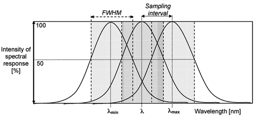
Figure 9. Adapted from (Van der Meer and De Jong, Citation2011). Inter-band Pearson’s linear cross-correlation (PLCC) coefficient, in range [−1.0, 1.0] (Kreyszig, Citation1979; Sheskin, Citation2000; Tabachnick & Fidell, Citation2014), for the main factors resulting from a principal component analysis and factor rotation for an agricultural data set acquired by the 220-band Jet Propulsion Laboratory (JPL) 220-band Airborne Visible Near Infrared Imaging Spectrometer (AVIRIS). Flevoland test site, July 5th 1991. It shows that, a global image-wide inter-band PLCC estimate, where typical local image non-stationarities are lost (Egorov, Roy, Zhang, Hansen, and Kommareddy, Citation2018) because averaged (wiped out), according to the central limit theorem (Kreyszig, Citation1979; Sheskin, Citation2000; Tabachnick & Fidell, Citation2014), scores (fuzzy) “high” (close to 1) within each of the three portions of the electromagnetic spectrum, namely, visible (VIS) ∈ [0.35 μm, 0.72 μm], Near-Infrared (NIR) ∈ [0.72 μm, 1.30 μm] and Middle-Infrared (MIR) ∈ [1.30 μm, 3.00 μm), see .
![Figure 9. Adapted from (Van der Meer and De Jong, Citation2011). Inter-band Pearson’s linear cross-correlation (PLCC) coefficient, in range [−1.0, 1.0] (Kreyszig, Citation1979; Sheskin, Citation2000; Tabachnick & Fidell, Citation2014), for the main factors resulting from a principal component analysis and factor rotation for an agricultural data set acquired by the 220-band Jet Propulsion Laboratory (JPL) 220-band Airborne Visible Near Infrared Imaging Spectrometer (AVIRIS). Flevoland test site, July 5th 1991. It shows that, a global image-wide inter-band PLCC estimate, where typical local image non-stationarities are lost (Egorov, Roy, Zhang, Hansen, and Kommareddy, Citation2018) because averaged (wiped out), according to the central limit theorem (Kreyszig, Citation1979; Sheskin, Citation2000; Tabachnick & Fidell, Citation2014), scores (fuzzy) “high” (close to 1) within each of the three portions of the electromagnetic spectrum, namely, visible (VIS) ∈ [0.35 μm, 0.72 μm], Near-Infrared (NIR) ∈ [0.72 μm, 1.30 μm] and Middle-Infrared (MIR) ∈ [1.30 μm, 3.00 μm), see Figure 7.](/cms/asset/fe48e3a3-184a-4435-bcd0-26afcfe6c83d/tbed_a_2017549_f0009_c.jpg)
Figure 10. In a new notion of Space Economy 4.0, envisioned by Mazzucato and Robinson in 2017 in their original work for the European Space Agency (ESA) (Mazzucato & Robinson, Citation2017), first-stage “horizontal” (enabling) capacity building, coping with background conditions necessary to specialization, is preliminary to second-stage “vertical” (deep and narrow) specialization policies, suitable for coping with a potentially huge worldwide market of institutional and private end-users of space technology. Definitions adopted herein, in agreement with the new notion of Space Economy 4.0 proposed by Mazzucato and Robinson (Mazzucato & Robinson, Citation2017), are: Space segment, Upstream segment for «mission control» = Ground segment for «mission control», Ground segment for «user support» = Midstream segment infrastructures and services, Downstream segment = Downstream utility of space technology (Mazzucato & Robinson, Citation2017, pp. 6, 57), capable of transforming quantitative (unequivocal) Earth observation (EO) big sensory data into sensory data-derived value-adding information products and services (VAPS), suitable for use by a potentially huge worldwide market of institutional and private end-users of space technology. Artificial General Intelligence (AGI) for EO (AGI4EO) technologies should be applied as early as possible in the “seamless innovation chain” required by a new notion of Space Economy 4.0, starting from AGI for space segment (AGI4Space) applications, which include the notion of future intelligent EO satellites, provided with AGI onboard (EOportal, Citation2020; ESA – European Space Agency, Citation2019; Esposito et al., Citation2019a, Citation2019b; GISCafe News, Citation2018; Zhou, Citation2001), and AGI for Data and Information Access Services (AGI4DIAS) at the midstream segment (see ), such as systematic generation of multi-sensor Analysis Ready Data (ARD) and information products, eligible for direct use in analysis at the downstream segment, without requiring laborious data pre-processing (Baraldi & Tiede, Citation2018a, Citation2018b; CEOS – Committee on Earth Observation Satellites, Citation2018; Dwyer et al., Citation2018; Helder et al., Citation2018; NASA – National Aeronautics and Space Administration, Citation2019; Qiu et al., Citation2019; USGS – U.S. Geological Survey, Citation2018a, Citation2018c).
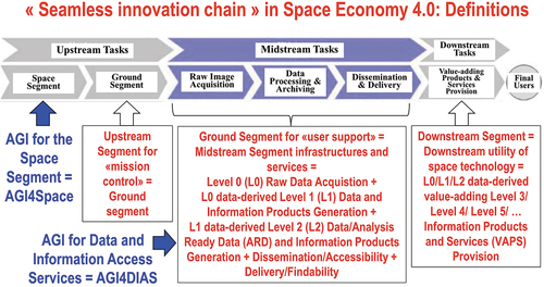
Figure 11. (a) Adapted from (Baraldi, Citation2017; Baraldi & Tiede, Citation2018a, Citation2018b), this original graph postulates that, within the multi-disciplinary cognitive science domain (Ball, Citation2021; Capra & Luisi, Citation2014; Hassabis et al., Citation2017; Hoffman, Citation2008, Citation2014; Langley, Citation2012; Miller, Citation2003; Mindfire Foundation, Citation2018; Mitchell, Citation2019; Parisi, Citation1991; Santoro et al., Citation2021; Serra & Zanarini, Citation1990; Varela et al., Citation1991; Wikipedia, Citation2019), encompassing disciplines like philosophy (Capurro & Hjørland, Citation2003; Dreyfus, Citation1965, Citation1991, Citation1992; Fjelland, Citation2020), semiotics (Ball, Citation2021; Peirce, Citation1994; Perez, Citation2020, Citation2021; Salad, Citation2019; Santoro et al., Citation2021; Wikipedia, Citation2021e), linguistics (Ball, Citation2021; Berlin & Kay, Citation1969; Firth, Citation1962; Rescorla, Citation2019; Saba, Citation2020a, Citation2020c), anthropology (Harari, Citation2011, Citation2017; Wikipedia, Citation2019), neuroscience (Barrett, Citation2017; Buonomano, Citation2018; Cepelewicz, Citation2021; Hathaway, Citation2021; Hawkins, Citation2021; Hawkins, Ahmad, and Cui, Citation2017; Kaufman, Churchland, Ryu, and Shenoy, Citation2014; Kosslyn, Citation1994; Libby & Buschman, Citation2021; Mason & Kandel, Citation1991; Salinas, Citation2021b; Slotnick et al., Citation2005; Zador, Citation2019), focusing on the study of the brain machinery in the mind-brain problem (Hassabis et al., Citation2017; Hoffman, Citation2008; Serra & Zanarini, Citation1990; Westphal, Citation2016), computational neuroscience (Beniaguev et al., Citation2021; DiCarlo, Citation2017; Gidon et al., Citation2020; Heitger et al., Citation1992; Pessoa, Citation1996; Rodrigues & Du Buf, Citation2009), psychophysics (Benavente et al., Citation2008; Bowers & Davis, Citation2012; Griffin, Citation2006; Lähteenlahti, Citation2021; Mermillod et al., Citation2013; Parraga et al., Citation2009; Vecera & Farah, Citation1997), psychology (APS – Association for Psychological Science, Citation2008; Hehe, Citation2021) computer science, formal logic (Laurini & Thompson, Citation1992; Sowa, Citation2000), mathematics, physics, statistics and (the meta-science of) engineering (Langley, Citation2012; Santoro et al., Citation2021; Wikipedia, Citation2019), semantic relationship ‘Human vision → Computer Vision (CV) ⊃ Earth observation (EO) image understanding (EO-IU)’ = EquationEquation (4)(4)
(4) holds true, where symbol ‘→’ denotes semantic relationship part-of (without inheritance) pointing from the supplier to the client, not to be confused with relationship subset-of, ‘⊃’, meaning specialization with inheritance from the superset (at left) to the subset, in agreement with symbols adopted by the standard Unified Modeling Language (UML) for graphical modeling of object-oriented software (Fowler, Citation2003). The working hypothesis ‘Human vision → CV ⊃ EO-IU’ = EquationEquation (4)
(4)
(4) means that human vision is expected to work as lower bound of CV, i.e. a CV system is required to include as part-of a computational model of human vision (Baraldi, Citation2017; Baraldi et al., Citation2018a, Citation2018b; Baraldi & Tiede, Citation2018a, Citation2018b; Iqbal & Aggarwal, Citation2001), consistent with human visual perception, in agreement with a reverse engineering approach to CV (Baraldi, Citation2017; Bharath & Petrou, Citation2008; DiCarlo, Citation2017). In practice, to become better conditioned for numerical solution (Baraldi, Citation2017; Baraldi et al., Citation2018a, Citation2018b; Baraldi & Tiede, Citation2018a, Citation2018b; Bishop, Citation1995; Cherkassky & Mulier, Citation1998; Dubey, Agrawal, Pathak, Griffiths, & Efros, Citation2018), an inherently ill-posed CV system is required to comply with human visual perception phenomena in the multi-disciplinary domain of cognitive science. (b) In this original graph, the inherently vague/equivocal notion of Artificial Intelligence is disambiguated into the two concepts of Artificial General Intelligence (AGI) and Artificial Narrow Intelligence (ANI), which are better constrained to be better understood (Bills, Citation2020; Chollet, Citation2019; Dreyfus, Citation1965, Citation1991, Citation1992; EC – European Commission, Citation2019; Fjelland, Citation2020; Hassabis et al., Citation2017; Ideami, Citation2021; Jajal, Citation2018; Mindfire Foundation, Citation2018; Practical AI, Citation2020; Santoro et al., Citation2021; Sweeney, Citation2018a; Wolski, Citation2020a, Citation2020b). This graph postulates that semantic relationship ‘EO-IU ⊂ CV ⊂ Artificial General Intelligence (AGI) ← Artificial Narrow Intelligence (ANI) ← (Inductive/ bottom-up/ statistical model-based) Machine Learning-from-data (ML) ⊃ (Inductive/ bottom-up/ statistical model-based) Deep Learning-from-data (DL)’ = ‘EO-IU ⊂ CV ⊂ AGI ← ANI ← ML ⊃ DL’ = EquationEquation (5)
(5)
(5) holds, where ANI is formulated as ‘ANI = [DL ⊂ ML logical-OR Traditional deductive Artificial Intelligence (static expert systems, non-adaptive to data, often referred to as Good Old-Fashioned Artificial Intelligence, GOFAI (Dreyfus, Citation1965, Citation1991, Citation1992; Santoro et al., Citation2021)]’ = EquationEquation (6)
(6)
(6) , in agreement with the entity-relationship model shown in (a). (c) In recent years, an increasingly popular thesis is that semantic relationship ‘A(G/N)I ⊃ ML ⊃ DL’ = EquationEquation (7)
(7)
(7) holds (Claire, Citation2019; Copeland, Citation2016). For example, in (Copeland, Citation2016), it is reported that: “since an early flush of optimism in the 1950s, smaller subsets of Artificial Intelligence – first machine learning, then deep learning, a subset of machine learning – have created even larger disruptions.” It is important to stress that the increasingly popular postulate (axiom) ‘A(G/N)I ⊃ ML ⊃ DL’ = EquationEquation (7)
(7)
(7) (Claire, Citation2019; Copeland, Citation2016), see Figure 11(c), is inconsistent with (alternative to) semantic relationship ‘AGI ← ANI ← ML ⊃ DL’ = EquationEquation (5)
(5)
(5) , depicted in Figure 11(a) and Figure 11(b). The latter is adopted as working hypothesis by the present paper.
![Figure 11. (a) Adapted from (Baraldi, Citation2017; Baraldi & Tiede, Citation2018a, Citation2018b), this original graph postulates that, within the multi-disciplinary cognitive science domain (Ball, Citation2021; Capra & Luisi, Citation2014; Hassabis et al., Citation2017; Hoffman, Citation2008, Citation2014; Langley, Citation2012; Miller, Citation2003; Mindfire Foundation, Citation2018; Mitchell, Citation2019; Parisi, Citation1991; Santoro et al., Citation2021; Serra & Zanarini, Citation1990; Varela et al., Citation1991; Wikipedia, Citation2019), encompassing disciplines like philosophy (Capurro & Hjørland, Citation2003; Dreyfus, Citation1965, Citation1991, Citation1992; Fjelland, Citation2020), semiotics (Ball, Citation2021; Peirce, Citation1994; Perez, Citation2020, Citation2021; Salad, Citation2019; Santoro et al., Citation2021; Wikipedia, Citation2021e), linguistics (Ball, Citation2021; Berlin & Kay, Citation1969; Firth, Citation1962; Rescorla, Citation2019; Saba, Citation2020a, Citation2020c), anthropology (Harari, Citation2011, Citation2017; Wikipedia, Citation2019), neuroscience (Barrett, Citation2017; Buonomano, Citation2018; Cepelewicz, Citation2021; Hathaway, Citation2021; Hawkins, Citation2021; Hawkins, Ahmad, and Cui, Citation2017; Kaufman, Churchland, Ryu, and Shenoy, Citation2014; Kosslyn, Citation1994; Libby & Buschman, Citation2021; Mason & Kandel, Citation1991; Salinas, Citation2021b; Slotnick et al., Citation2005; Zador, Citation2019), focusing on the study of the brain machinery in the mind-brain problem (Hassabis et al., Citation2017; Hoffman, Citation2008; Serra & Zanarini, Citation1990; Westphal, Citation2016), computational neuroscience (Beniaguev et al., Citation2021; DiCarlo, Citation2017; Gidon et al., Citation2020; Heitger et al., Citation1992; Pessoa, Citation1996; Rodrigues & Du Buf, Citation2009), psychophysics (Benavente et al., Citation2008; Bowers & Davis, Citation2012; Griffin, Citation2006; Lähteenlahti, Citation2021; Mermillod et al., Citation2013; Parraga et al., Citation2009; Vecera & Farah, Citation1997), psychology (APS – Association for Psychological Science, Citation2008; Hehe, Citation2021) computer science, formal logic (Laurini & Thompson, Citation1992; Sowa, Citation2000), mathematics, physics, statistics and (the meta-science of) engineering (Langley, Citation2012; Santoro et al., Citation2021; Wikipedia, Citation2019), semantic relationship ‘Human vision → Computer Vision (CV) ⊃ Earth observation (EO) image understanding (EO-IU)’ = EquationEquation (4)(4) \lsquo(Inductive/ bottom-up/ statistical model-based) DL-from-data⊂(Inductive/ bottom-up / statistical model-based) ML-from-data→AGI⊃CV←Human vision\rsquo(4) holds true, where symbol ‘→’ denotes semantic relationship part-of (without inheritance) pointing from the supplier to the client, not to be confused with relationship subset-of, ‘⊃’, meaning specialization with inheritance from the superset (at left) to the subset, in agreement with symbols adopted by the standard Unified Modeling Language (UML) for graphical modeling of object-oriented software (Fowler, Citation2003). The working hypothesis ‘Human vision → CV ⊃ EO-IU’ = EquationEquation (4)(4) \lsquo(Inductive/ bottom-up/ statistical model-based) DL-from-data⊂(Inductive/ bottom-up / statistical model-based) ML-from-data→AGI⊃CV←Human vision\rsquo(4) means that human vision is expected to work as lower bound of CV, i.e. a CV system is required to include as part-of a computational model of human vision (Baraldi, Citation2017; Baraldi et al., Citation2018a, Citation2018b; Baraldi & Tiede, Citation2018a, Citation2018b; Iqbal & Aggarwal, Citation2001), consistent with human visual perception, in agreement with a reverse engineering approach to CV (Baraldi, Citation2017; Bharath & Petrou, Citation2008; DiCarlo, Citation2017). In practice, to become better conditioned for numerical solution (Baraldi, Citation2017; Baraldi et al., Citation2018a, Citation2018b; Baraldi & Tiede, Citation2018a, Citation2018b; Bishop, Citation1995; Cherkassky & Mulier, Citation1998; Dubey, Agrawal, Pathak, Griffiths, & Efros, Citation2018), an inherently ill-posed CV system is required to comply with human visual perception phenomena in the multi-disciplinary domain of cognitive science. (b) In this original graph, the inherently vague/equivocal notion of Artificial Intelligence is disambiguated into the two concepts of Artificial General Intelligence (AGI) and Artificial Narrow Intelligence (ANI), which are better constrained to be better understood (Bills, Citation2020; Chollet, Citation2019; Dreyfus, Citation1965, Citation1991, Citation1992; EC – European Commission, Citation2019; Fjelland, Citation2020; Hassabis et al., Citation2017; Ideami, Citation2021; Jajal, Citation2018; Mindfire Foundation, Citation2018; Practical AI, Citation2020; Santoro et al., Citation2021; Sweeney, Citation2018a; Wolski, Citation2020a, Citation2020b). This graph postulates that semantic relationship ‘EO-IU ⊂ CV ⊂ Artificial General Intelligence (AGI) ← Artificial Narrow Intelligence (ANI) ← (Inductive/ bottom-up/ statistical model-based) Machine Learning-from-data (ML) ⊃ (Inductive/ bottom-up/ statistical model-based) Deep Learning-from-data (DL)’ = ‘EO-IU ⊂ CV ⊂ AGI ← ANI ← ML ⊃ DL’ = EquationEquation (5)(5) \lsquoARD⊂EO-IU⊂CV⊂AGI←ANI←ML⊃DL⊃DeepConvolutionalNeuralNetworkDCNN\rsquo(5) holds, where ANI is formulated as ‘ANI = [DL ⊂ ML logical-OR Traditional deductive Artificial Intelligence (static expert systems, non-adaptive to data, often referred to as Good Old-Fashioned Artificial Intelligence, GOFAI (Dreyfus, Citation1965, Citation1991, Citation1992; Santoro et al., Citation2021)]’ = EquationEquation (6)(6) x0026;ANI=[DCNN⊂DL⊂MLlogical0ORTraditionaldeductiveArtificial Intelligencex0026;(staticexpertsystems,non0adaptivetodata,alsoknownasGoodOld0Fashionedx0026;Artificial Intelligence,GOFAI](6) , in agreement with the entity-relationship model shown in (a). (c) In recent years, an increasingly popular thesis is that semantic relationship ‘A(G/N)I ⊃ ML ⊃ DL’ = EquationEquation (7)(7) \lsquoA(G/N)I⊃ML⊃DL⊃DCNN\rsquo(7) holds (Claire, Citation2019; Copeland, Citation2016). For example, in (Copeland, Citation2016), it is reported that: “since an early flush of optimism in the 1950s, smaller subsets of Artificial Intelligence – first machine learning, then deep learning, a subset of machine learning – have created even larger disruptions.” It is important to stress that the increasingly popular postulate (axiom) ‘A(G/N)I ⊃ ML ⊃ DL’ = EquationEquation (7)(7) \lsquoA(G/N)I⊃ML⊃DL⊃DCNN\rsquo(7) (Claire, Citation2019; Copeland, Citation2016), see Figure 11(c), is inconsistent with (alternative to) semantic relationship ‘AGI ← ANI ← ML ⊃ DL’ = EquationEquation (5)(5) \lsquoARD⊂EO-IU⊂CV⊂AGI←ANI←ML⊃DL⊃DeepConvolutionalNeuralNetworkDCNN\rsquo(5) , depicted in Figure 11(a) and Figure 11(b). The latter is adopted as working hypothesis by the present paper.](/cms/asset/b29472e6-c5ea-4c54-b733-1ccd114b1b34/tbed_a_2017549_f0011a_c.jpg)
Figure 11. Continued.
Figure 12. Adapted from (Wikipedia, Citation2020a). The increasingly popular Data-Information-Knowledge-Wisdom (DIKW) pyramid (Rowley, Citation2007; Rowley & Hartley, Citation2008; Wikipedia, Citation2020a; Zeleny, Citation1987, Citation2005; Zins, Citation2007), also known as the DIKW hierarchy, refers loosely to a class of models for representing purported structural and/or functional relationships between data, information, knowledge, and wisdom (Zins, Citation2007). Typically, “information is defined in terms of data, knowledge in terms of information and wisdom in terms of knowledge” (Rowley, Citation2007; Rowley & Hartley, Citation2008).

Figure 13. Hyperparameter tuning for model optimization and the bias-variance trade-off (Bishop, Citation1995; Cherkassky & Mulier, Citation1998; Geman et al., Citation1992; Koehrsen, Citation2018; Mahadevan, Citation2019; Sarkar, Citation2018; Wikipedia, Citation2010; Wolpert, Citation1996; Wolpert & Macready, Citation1997). As a general rule, “proper feature engineering will have a much larger impact on model performance than even the most extensive hyperparameter tuning. It is the law of diminishing returns applied to machine learning: feature engineering gets you most of the way there, and hyperparameter tuning generally only provides a small benefit. This demonstrates a fundamental aspect of machine learning: it is always a game of trade-offs. We constantly have to balance accuracy vs interpretability, bias vs variance, accuracy vs run time, and so on” (Koehrsen, Citation2018). On the one hand, “if you shave off your hypothesis with a big Occam’s razor, you will be likely left with a simple model, one which cannot fit all the data. Consequently, you have to supply more data to have better confidence. On the other hand, if you create a complex (and long) hypothesis, you may be able to fit your training data really well (low bias, low error rate), but this actually may not be the right hypothesis as it runs against the maximum a posteriori (MAP) principle of having a hypothesis with small entropy (with Entropy = -log2P(Hypothesis) = length(Hypothesis)) in addition to a small error rate” (Sarkar, Citation2018).
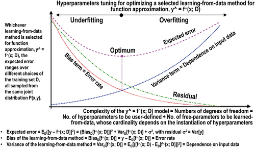
Figure 14. Adapted from (Koehrsen, Citation2018). The so-called “black box problem” closes in on machine learning (ML)-from-data algorithms in general. In artificial neural networks (ANNs), typically based on the McCulloch and Pitts (MCP) neuron model, conceived almost 80 years ago as a simplified neurophysiological version of biological neurons (McCulloch & Pitts, Citation1943), or its improved recent versions (Cimpoi et al., Citation2014; Krizhevsky et al., Citation2012), in compliance with the mind-brain problem (Hassabis et al., Citation2017; Hoffman, Citation2008; Serra & Zanarini, Citation1990; Westphal, Citation2016), the difficulty for the system to provide a suitable explanation for how it arrived at an answer is referred to as “the black box problem”, which affects how an ANN can hit the point of reproducibility or at least traceability/interpretability (Koehrsen, Citation2018; Lukianoff, Citation2019). This chart shows “a (highly unscientific) version of the accuracy vs interpretability trade-off, to highlight a fundamental aspect of ML: it is always a game of trade-offs. We constantly have to balance accuracy vs interpretability, bias vs variance, accuracy vs run time, and so on” (Koehrsen, Citation2018), also refer to .
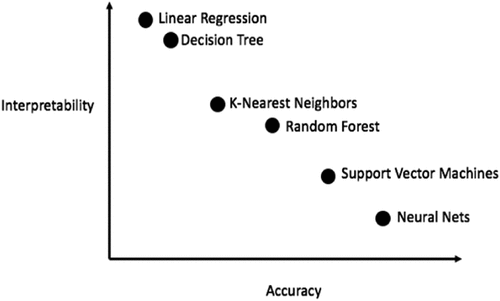
Figure 15. Example of latent/hidden variable as a discrete and finite vocabulary of basic color (BC) names (Baraldi & Tiede, Citation2018a, Citation2018b; berlin & Kay, Citation1969; Griffin, Citation2006). This graphical model of color naming is adapted from (Shotton, Winn, Rother, & Criminisi, Citation2009; Wikipedia, Citation2015). Let us consider z as a (subsymbolic) numerical variable, such as multi-spectral (MS) color values of a population of spatial units belonging to a (2D) image-plane, where spatial units can be either (0D) pixel, (1D) line or (2D) polygon (OGC – Open Geospatial Consortium Inc, Citation2015), with vector data z ∈ ℜMS, where ℜMS represents a multi-spectral (MS) data space, while c represents a categorical variable of symbolic classes in the 4D geospace-time scene-domain, pertaining to the physical real-world, with c = 1, …, ObjectClassLegendCardinality. (a) According to Bayesian theory, posterior probability , where color names ks, equivalent to color (hyper)polyhedra (Benavente et al., Citation2008; Griffin, Citation2006; Parraga et al., Citation2009) in a numerical color (hyper)space ℜMS, provide a partition of the domain of change, ℜMS, of numerical variable z (refer to the farther Figure 29). (b) For discriminative inference, the arrows in the graphical model are reversed using Bayes rule. Hence, a vocabulary of color names, physically equivalent to a partition of a numerical color space ℜMS into color name-specific hyperpolyhedra, is conceptually equivalent to a latent/ hidden/ hypothetical variable linking observables (subsymbolic sensory data) in the real world, specifically, color values, to a categorical variable of semantic (symbolic) quality in the mental (conceptual) model of the physical world (world ontology, world model) (Baraldi, Citation2017; Baraldi & Tiede, Citation2018a, Citation2018b; Matsuyama & Hwang, Citation1990).
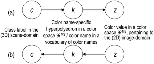
Figure 16. Augmented (better constrained) version of the traditional Data-Information-Knowledge-Wisdom (DIKW) pyramid (Rowley, Citation2007; Rowley and Hartley, Citation2008; Wikipedia, Citation2020a; Zeleny, Citation1987; Zeleny, Citation2005; Zins, Citation2007) (see ), where “information is typically defined in terms of data, knowledge in terms of information, and wisdom in terms of knowledge” (Rowley, Citation2007). Intuitively, Zeleny defines knowledge as “know-how” (procedural knowledge) (Saba, Citation2020b) and wisdom as “what to do, act or carry out”/know-what and “why do”/know-why (Zeleny, Citation1987; Zeleny, Citation2005). The conceptual and factual gap between knowledge as “know-how” (factual statement) (Harari, Citation2017, p. 222) and wisdom as “what to do”/know-what and “why do”/know-why (ethical judgement) (Harari, Citation2017, p. 222) is huge to be filled by any human-like Artificial General Intelligence (AGI), capable of human personal and collective (societal) intelligence (Benavente, Vanrell, and Baldrich, Citation2008; Harari, Citation2017). This is acknowledged by Yuval Noah Harari, who writes: filling the gap from knowledge as “know-how” (factual statement) to wisdom as “what to do”/know-what and “why do”/know-why (ethical judgement) is equivalent to crossing “the border from the land of science into that of religion” (Harari, Citation2017, p. 244). About the relationship between religion and science, “science always needs religious assistance in order to create viable human institutions. Scientists study how the world functions, but there is no scientific method for determining how humans ought to behave. Only religions provide us with the necessary guidance” (Harari, Citation2017, p. 219).
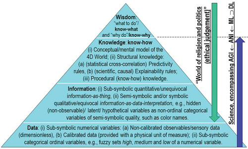
Figure 17. Adapted from (Camara, Citation2017). Google Trends: Big data vs Machine learning (ML) search trends, May 6, 2012 – May 6, 2017.
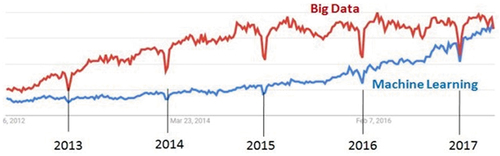
Figure 18. Lesson to be learned from big data analysis, required to cope with the six Vs of volume, velocity, variety, veracity, volatility and value (Metternicht et al., Citation2020). For example, the popular Google Earth Engine (Gorelick et al., Citation2017) is typically considered a valuable instance of the set of algorithms suitable for working on EO large image databases. Noteworthy, the Google Earth Engine typically adopts a pixel-based-through-time image analysis approach, synonym for spatial-context insensitive 1D image analysis. The computer vision (CV) and remote sensing (RS) communities have been striving to abandon 1D analysis of (2D) imagery since the 1970s (Nagao & Matsuyama, Citation1980). In spite of these efforts, to date, in the RS common practice, traditional suboptimal algorithms for 1D analysis of (2D) imagery implemented in the Google Earth Engine platform are considered the state-of-the-art in EO big data cube analysis (Gorelick et al., Citation2017). Only a small subset of data processing algorithms scores “(fuzzy) high” in a minimally dependent maximally informative (mDMI) set of outcome and process quantitative quality indicators (OP-Q2Is), including accuracy, efficiency, robustness to changes in input data, robustness to changes in input parameters, scalability, timeliness, costs and value (Baraldi, Citation2017; Baraldi & Boschetti, Citation2012a, Citation2012b; Baraldi et al., Citation2014, Citation2018a, Citation2018b; Baraldi & Tiede, Citation2018a, Citation2018b) (refer to Subsection 3.1), in both small data analysis and big data analysis. Only this small subset of data processing algorithms belongs to the domain of interest of Artificial General Intelligence (AGI) = EquationEquation (5)(5)
(5) , see .
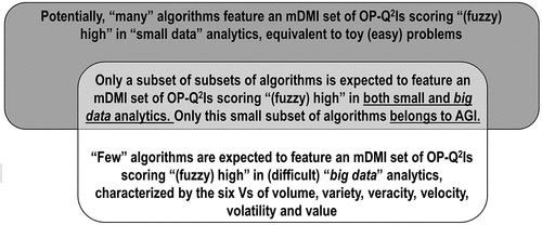
Figure 19. (a) Adapted from (Manilici et al., Citation2013). Deutsches Zentrum für Luft- und Raumfahrt (German Aerospace Center, DLR) archive size in petabytes (PB) of optical and synthetic aperture radar (SAR) data acquired by spaceborne imaging sensors. Status on July 30, 2013. Also refer to (Belward & Skøien, Citation2015; NASA – National Aeronautics and Space Administration, Citation2016; Pinna & Ferrante, Citation2009). (b) Global European annual satellite EO products and services turnover, in millions of euros (eoVox, Citation2008). Unfortunately, this latter estimate, which is monotonically increasing with the number of EO data users, provides no clue at all on the average per user productivity, monotonically increasing with the average number of different EO images actually used (interpreted, rather than downloaded) by a single user per year. Our conjecture is that existing suboptimal EO image understanding (EO-IU) systems, not provided with the Artificial General Intelligence (AGI) capability required to accomplish EO big data interpretation in operational mode (see ), have been outpaced in productivity by the exponential rate of collection of EO sensory data, whose quality and quantity are ever-increasing, see .
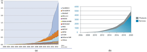
Figure 20. Synonym for scene-from-image reconstruction and understanding (Matsuyama & Hwang, Citation1990), vision is a cognitive problem (Ball, Citation2021; Capra & Luisi, Citation2014; Hassabis et al., Citation2017; Hoffman, Citation2008, Citation2014; Langley, Citation2012; Miller, Citation2003; Mindfire Foundation, Citation2018; Mitchell, Citation2019; Parisi, Citation1991; Santoro et al., Citation2021; Serra & Zanarini, Citation1990; Varela et al., Citation1991; Wikipedia, Citation2019), i.e. it is an inherently qualitative/ equivocal/ ill-posed information-as-data-interpretation task (Baraldi, Citation2017; Baraldi et al., Citation2018a, Citation2018b; Baraldi & Tiede, Citation2018a, Citation2018b; Capurro & Hjørland, Citation2003), see . Encompassing both biological vision and computer vision (CV) (see ), vision is very difficult to solve because: (i) non-deterministic polynomial (NP)-hard in computational complexity (Frintrop, Citation2011; Tsotsos, Citation1990), and (ii) inherently ill-posed in the Hadamard sense (Baraldi, Citation2017; Baraldi & Tiede, Citation2018a, Citation2018b; Hadamard, Citation1902; Matsuyama & Hwang, Citation1990) (refer to Section 2). Vision is inherently ill-posed because affected by: (a) a 4D-to-2D data dimensionality reduction, from the 4D geospatio-temporal scene-domain to the (2D, planar) image-domain, which is responsible of occlusion phenomena, and (b) a semantic information gap (Matsuyama & Hwang, Citation1990), from ever-varying subsymbolic sensory data (sensations) in the physical world-domain to stable symbolic percepts in the mental model of the physical world (modeled world, world ontology, real-world model). Since it is inherently ill-posed, vision requires a priori knowledge in addition to sensory data to become better posed for numerical solution (Baraldi, Citation2017; Baraldi et al., Citation2018a, Citation2018b; Baraldi & Tiede, Citation2018a, Citation2018b; Bishop, Citation1995; Cherkassky & Mulier, Citation1998; Dubey et al., Citation2018).
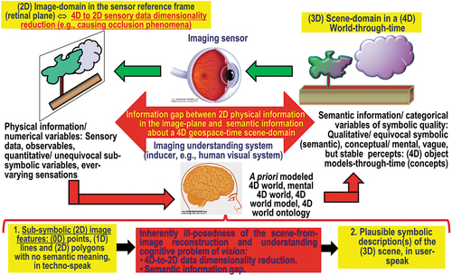
Figure 21. An observation (true-fact) familiar to all human beings wearing sunglasses, such as “spatial information dominates color information in vision” (Baraldi, Citation2017; Baraldi et al., Citation2018a, Citation2018b; Baraldi & Tiede, Citation2018a, Citation2018b), is typically questioned or disagreed upon by many computer vision (CV) and remote sensing (RS) experts and/or practitioners. At right, a panchromatic Baboon is as easy to be visually identified as such as its chromatic counterpart, at left, by any human photointerpreter. This perceptual fact works as proof-of-concept that the bulk of visual information is spatial rather than colorimetric in both the 4D geospace-time scene-domain and its projected (2D) image-plane. In spite of this unequivocal true-fact, to date, the great majority of the CV and RS communities adopt 1D non-retinotopic/2D spatial topology non-preserving (Baraldi, Citation2017; Baraldi & Alpaydin, Citation2002a, Citation2002b; Fritzke, Citation1997; Martinetz et al., Citation1994; Öğmen & Herzog, Citation2010; Tsotsos, Citation1990) image analysis algorithms, either pixel-based or local window-based, insensitive to permutations in the input data sequence (Cimpoi et al., Citation2014; Krizhevsky et al., Citation2012), where inter-object spatial topological relationships (e.g. adjacency, inclusion, etc.) and inter-object spatial non-topological relationships (e.g. spatial distance and angle measure) are oversighted in the (2D) image-plane (refer to Subsection 3.3.4), also refer to .
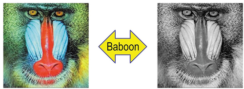
Figure 22. Examples of 1D image analysis approaches (Baraldi, Citation2017; Baraldi et al., Citation2018a, Citation2018b; Baraldi & Tiede, Citation2018a, Citation2018b; Matsuyama & Hwang, Citation1990), 2D spatial topology non-preserving (non-retinotopic) in the (2D) image-domain (Baraldi, Citation2017; Baraldi & Alpaydin, Citation2002a, Citation2002b; Fritzke, Citation1997; Martinetz et al., Citation1994; Öğmen & Herzog, Citation2010; Tsotsos, Citation1990). Intuitively, 1D image analysis is insensitive to permutations in the input data set (Cimpoi et al., Citation2014; Krizhevsky et al., Citation2012). Synonym for 1D analysis of a 2D gridded data set, non-retinotopic 1D image analysis is affected by spatial data dimensionality reduction, from 2D to 1D. The (2D) image at top/left is transformed into the 1D vector data stream (sequence) shown at bottom/right, where vector data are either pixel-based (2D spatial context-insensitive) or spatial context-sensitive, e.g. local window-based or image-object-based. This 1D vector data stream means nothing to a human photo interpreter. When it is input to either an inductive learning-from-data classifier or a deductive learning-by-rule classifier, the 1D vector data sequence is what the classifier actually sees when watching the (2D) image at left. Undoubtedly, computers are more successful than humans in 1D image analysis. Nonetheless, humans are still far more successful than computers in 2D image analysis, which is 2D spatial context-sensitive and 2D spatial topology-preserving (retinotopic) (Baraldi, Citation2017; Baraldi & Alpaydin, Citation2002a, Citation2002b; Fritzke, Citation1997; Martinetz et al., Citation1994; Öğmen & Herzog, Citation2010; Tsotsos, Citation1990), see . (a) Pixel-based (2D spatial context-insensitive) or (spatial context-sensitive) local window-based 1D image analysis. (b) Typical example of 1D image analysis approach implemented within the (geographic) object-based image analysis (GEOBIA) paradigm (Baraldi, Lang, Tiede, & Blaschke, Citation2018; Blaschke et al., Citation2014). In the so-called (GE)OBIA approach to CV, spatial analysis of (2D) imagery is intended to replace traditional pixel-based/2D spatial context-insensitive image analysis algorithms, dominating the RS literature to date. In practice, (GE)OBIA solutions can pursue either (2D spatial topology non-preserving, non-retinotopic) 1D image analysis or (2D spatial topology preserving, retinotopic) 2D image analysis (Baraldi et al., Citation2018). Also refer to and .
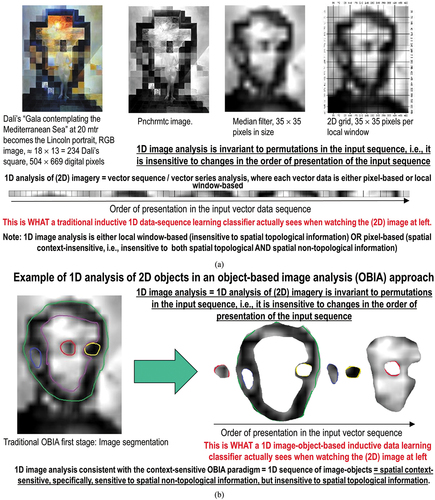
Figure 23. Alternative to 1D analysis of (2D) imagery (see .), image analysis (Baraldi, Citation2017; Baraldi et al., Citation2018a, Citation2018b; Baraldi & Tiede, Citation2018a, Citation2018b; DiCarlo, Citation2017; Öğmen & Herzog, Citation2010; Tsotsos, Citation1990) is synonym for 2D analysis of (2D) imagery, meaning 2D spatial context-sensitive and 2D spatial topology-preserving (retinotopic) feature mapping in a (2D) image-domain (Baraldi, Citation2017; Baraldi & Alpaydin, Citation2002a, Citation2002b; Fritzke, Citation1997; Martinetz et al., Citation1994; Öğmen & Herzog, Citation2010; Tsotsos, Citation1990). Intuitively, 2D image analysis is sensitive to permutations in the input data set (Cimpoi et al., Citation2014; Krizhevsky et al., Citation2012). Activation domains of physically adjacent processing units in the 2D array (grid, network) of 2D convolutional spatial filters are spatially adjacent regions in the 2D visual field (image-plane). Distributed processing systems capable of 2D image analysis, such as physical model-based (‘handcrafted’) 2D wavelet filter banks (Baraldi, Citation2017; Burt & Adelson, Citation1983; DiCarlo, Citation2017; Jain & Healey, Citation1998; Mallat, Citation2009; Marr, Citation1982; Sonka et al., Citation1994), typically provided with a high degree of biological plausibility in modelling 2D spatial topological and spatial non-topological information components (DiCarlo, Citation2017; Heitger et al., Citation1992; Kosslyn, Citation1994; Mason & Kandel, Citation1991; Öğmen & Herzog, Citation2010; Rappe, Citation2018; Rodrigues & Du Buf, Citation2009; Slotnick et al., Citation2005; Tsotsos, Citation1990; Vecera & Farah, Citation1997) and/or deep convolutional neural networks (DCNNs), typically learned inductively (bottom-up) from data end-to-end (Cimpoi et al., Citation2014; Krizhevsky et al., Citation2012), are eligible for outperforming traditional 1D image analysis approaches. Will computer vision (CV) systems ever become as good as humans in 2D image analysis? Also refer to . Unfortunately, due to bad practices in multi-scale spatial filtering implementation (Geirhos et al., Citation2018; Zhang, Citation2019), modern inductive DCNN algorithms typically neglect the spatial ordering of object parts, i.e. they are insensitive to the shuffling of image parts (Brendel, Citation2019; Brendel & Bethge, Citation2019). In practice, large portions of modern inductive DCNNs adopt a decision-strategy very similar to that of traditional 1D image analysis approaches, such as bag-of-local-features models (Brendel, Citation2019; Brendel & Bethge, Citation2019), insensitive to permutations in the 1D sequence of input data (Bourdakos, Citation2017), see .
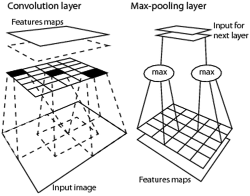
Figure 24. A (geographic) object-based image analysis (GEOBIA) paradigm (Blaschke et al., Citation2014), reconsidered (Baraldi et al., Citation2018). In the (GE)OBIA subdomain of computer vision (CV) (see ), spatial analysis of (2D) imagery is intended to replace traditional pixel-based (2D spatial context-insensitive) image analysis algorithms, dominating the remote sensing (RS) literature and common practice to date. In practice, (GE)OBIA solutions encompass either 1D image analysis (spatial topology non-preserving, non-retinotopic) or 2D image analysis (spatial topology preserving, retinotopic). To overcome limitations of the existing GEOBIA paradigm (Blaschke et al., Citation2014), in a more restrictive definition of EO for Geographic Information Science (GIScience) (EO4GIScience) (see ), novel EO4GIScience applications consider mandatory a 2D image analysis approach, see (Baraldi et al., Citation2018).
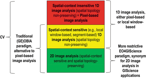
Figure 25. Adapted from (Bourdakos, Citation2017). Modern inductive learned-from-data end-to-end Deep Convolutional Neural Networks (DCNNs) typically neglect the spatial ordering of object parts, i.e. they are insensitive to the shuffling (permutations) of image parts. Hence, they are similar to traditional 1D image analysis approaches, such as bag-of-local-features models (Brendel, Citation2019; Brendel & Bethge, Citation2019). Experimental evidence and conclusions reported in (Brendel, Citation2019; Brendel & Bethge, Citation2019) are aligned with those reported in (Bourdakos, Citation2017). These experimental results highlight how little we have yet understood about the inner working of DCNNs. For example, a well-trained DCNN has difficulty with the concept of “correct face” whose parts, such as an eye and a mouth, are in the wrong place. In addition to being easily fooled by images with features in the wrong place, a DCNN is also easily confused when viewing an image in a different orientation. One way to combat this is with excessive training of all possible angles, but this takes a lot of time and seems counter intuitive (Bourdakos, Citation2017).
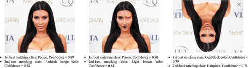
Figure 26. Adapted from (DiCarlo, Citation2017). As instance of the science of Natural Intelligence, reverse engineering primate visual perception adopts a stepwise approach (Baraldi, Citation2017; Bharath & Petrou, Citation2008; DiCarlo, Citation2017), in agreement with the seminal work by Marr (Marr, Citation1982).
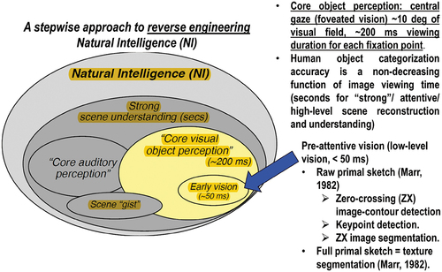
Figure 27. Mach bands visual illusion (Pessoa, Citation1996). Below, in the image profile, in black: Ramp in (true, quantitative) luminance units across space. In red: Brightness (qualitative, perceived luminance) across space, where brightness is defined as a subjective aspect of vision, i.e. brightness is the perceived luminance of a surface (Boynton, Citation1990). Where a luminance (radiance, intensity) ramp meets a plateau, there are spikes of brightness, although there is no discontinuity in the luminance profile. Hence, human vision detects two boundaries, one at the beginning and one at the end of the ramp in luminance, independent of the ramp slope. Since there is no discontinuity in luminance where brightness is spiking, the Mach bands effect is called a visual ‘illusion’. In the words of Luiz Pessoa, ‘if we require that a brightness model should at least be able to predict Mach bands, the bright and dark bands which are seen at ramp edges, the number of published models is surprisingly small’ (Pessoa, Citation1996). The important lesson to be learned from the Mach bands illusion is that, in vision, local variance, contrast and 1st-order derivative (gradient) are statistical features (data-derived numerical variables) computed locally in the (2D) image-domain not suitable to detect image-objects (segments, closed contours) required to be perceptually ‘uniform’ (‘homogeneous’) in agreement with human vision (Baraldi, Citation2017; Baraldi et al., Citation2018a, Citation2018b; Baraldi & Tiede, Citation2018a, Citation2018b; Iqbal & Aggarwal, Citation2001). In other words, these popular local statistics, namely, local variance, contrast and 1st-order derivative (gradient), are not suitable visual features if detected image-segments and/or image-contours are required to be consistent with human visual perception, including ramp-edge detection. This straightforward (obvious), but not trivial observation is at odd with a large portion of the existing computer vision (CV) and remote sensing (RS) literature, where many CV algorithms for semi-automatic image segmentation (Baatz & Schäpe, Citation2000; Camara et al., Citation1996; Espindola et al., Citation2006) or (vice versa) semi-automatic image-contour detection (Heitger et al., Citation1992), such as the popular Canny edge detector (Canny, Citation1986), are based on empirical thresholding the local variance, contrast or first-order gradient based on data-dependent heuristic criteria.
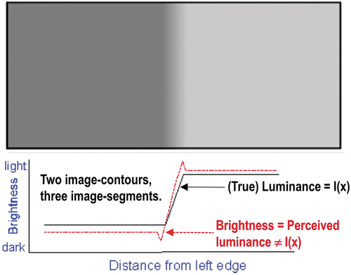
Figure 28. To comply with working hypothesis ‘Human vision → CV ⊃ EO-IU’ = EquationEquation (4)(4)
(4) (see ), a low-level ‘CV ⊃ EO-IU’ subsystem is implemented as a top-down/ deductive/ physical model-based (“handcrafted”) 2 grid (array) of wavelet-based multi-scale multi-orientation low-pass 2D Gaussian filters and band-pass trimodal even-symmetric 2D spatial filters (Baraldi, Citation2017). It is equivalent to a prior knowledge-based (physical model-based) deep convolutional neural network (DCNN), alternative to popular inductive DCNNs learned-from-data end-to-end (Cimpoi et al., Citation2014; Krizhevsky et al., Citation2012). Capable of automatic zero-crossing image-contour detection and image segmentation/partitioning, it complies with human visual perception (Baraldi, Citation2017; Baraldi et al., Citation2018a, Citation2018b; Baraldi & Tiede, Citation2018a, Citation2018b; Iqbal & Aggarwal, Citation2001), with regard to: (1) the Mach bands visual illusion (Pessoa, Citation1996) and (2) the perceptual true-fact that human panchromatic and chromatic vision mechanisms are nearly as effective in scene-from-image reconstruction and understanding. It is tested on complex spaceborne/airborne EO optical images in agreement with a stepwise approach, consistent with the property of systematicity of natural language/thought (Fodor, Citation1998; Peirce, Citation1994; Rescorla, Citation2019; Saba, Citation2020a) (refer to Subsection 3.4), to be regarded as commonsense knowledge, agreed upon by the entire human community (refer to Section 2). Testing images start from “simple” synthetic imagery of “known”, but challenging complexity in 2D spatial and colorimetric information components. If first-level testing with synthetic imagery is successful, next, natural panchromatic and RGB images, intuitive to cope with, are adopted for second-level testing purposes. Finally, complex spaceborne/airborne EO optical imagery, depicting manmade objects of known shape and size together with textured areas, are employed for third-level testing. (a) SUSAN synthetic panchromatic image, byte encoded in range {0, 255}, image size (rows × columns × bands) = 370 × 370 × 1. No histogram stretching applied for visualization purposes. Step edges and ramp edges at known locations (the latter forming the two inner rectangles visible at the bottom right corner) form angles from acute to obtuse. According to human vision, 31 image-segments can be detected as reference “ground-truth”. (b) Sum (synthesis) of the wavelet-based near-orthogonal multi-scale multi-orientation image decomposition. Filter value sum in range from −255.0 to +255.0. (c) Automated (requiring no human–machine interaction) image segmentation into zero-crossing segments generated from zero-crossing pixels detected by the multi-scale multi-orientation trimodal even-symmetric 2D spatial filter bank, different from Marr’s single-scale isotropic zero-crossing pixel detection (Marr, Citation1982). Exactly 31 image-segments are detected with 100% contour accuracy. Segment contours depicted with 8-adjacency cross-aura values in range {0, 8}, see . (d) Image-object mean view = object-wise constant input image reconstruction. No histogram stretching applied for visualization purposes. (e) Object-wise constant input image reconstruction compared with the input image, per-pixel root mean square error (RMSE) in range [0.0, 255.0], equivalent to a vector discretization/quantization (VQ) quality assessment in image decomposition (analysis, encoding) and reconstruction (synthesis, decoding) (Baraldi, Citation2017, Citation2019a; Baraldi et al., Citation2010a, Citation2010b, Citation2018a, Citation2018b, Citation2006; Baraldi & Tiede, Citation2018a, Citation2018b). (f) Natural panchromatic image of an actress wearing a Venetian carnival mask, image size (rows × columns × bands) = 438 × 310 × 1. No histogram stretching applied for visualization purposes. (g) Same as (b). (h) Same as (c), there is no CV system’s free- parameter to be user-defined. (i) Same as (d). (l) Same as (e). (m) Natural RGB-color image of an actress wearing a Venetian carnival mask, image size (rows × columns × bands) = 438 × 310 × 3. No histogram stretching applied for visualization purposes. (n) Same as (b). (o) Same as (c), there is no CV system’s free- parameter to be user-defined. (p) Same as (d). (q) Same as (e). (r) Zoom-in of a Sentinel-2A MSI Level-1 C image of the Earth surface south of the city of Salzburg, Austria. Acquired on 2015–09-11. Spatial resolution: 10 m. Radiometrically calibrated into top-of-atmosphere reflectance (TOARF) values in range [0.0, 1.0], byte-coded into range {0, 255}, it is depicted as a false color RGB image, where: R = Middle-InfraRed (MIR) = Band 11, G = Near IR (NIR) = Band 8, B = Blue = Band 2. Standard ENVI histogram stretching applied for visualization purposes. Image size (rows × columns × bands) = 545 × 660 × 3. (s) Same as (b). (t) Same as (c), there is no CV system’s free-parameter to be user-defined. (u) Same as (d), but now a standard ENVI histogram stretching is applied for visualization purposes. (v) Same as (e).
![Figure 28. To comply with working hypothesis ‘Human vision → CV ⊃ EO-IU’ = EquationEquation (4)(4) \lsquo(Inductive/ bottom-up/ statistical model-based) DL-from-data⊂(Inductive/ bottom-up / statistical model-based) ML-from-data→AGI⊃CV←Human vision\rsquo(4) (see Figure 11), a low-level ‘CV ⊃ EO-IU’ subsystem is implemented as a top-down/ deductive/ physical model-based (“handcrafted”) 2 grid (array) of wavelet-based multi-scale multi-orientation low-pass 2D Gaussian filters and band-pass trimodal even-symmetric 2D spatial filters (Baraldi, Citation2017). It is equivalent to a prior knowledge-based (physical model-based) deep convolutional neural network (DCNN), alternative to popular inductive DCNNs learned-from-data end-to-end (Cimpoi et al., Citation2014; Krizhevsky et al., Citation2012). Capable of automatic zero-crossing image-contour detection and image segmentation/partitioning, it complies with human visual perception (Baraldi, Citation2017; Baraldi et al., Citation2018a, Citation2018b; Baraldi & Tiede, Citation2018a, Citation2018b; Iqbal & Aggarwal, Citation2001), with regard to: (1) the Mach bands visual illusion (Pessoa, Citation1996) and (2) the perceptual true-fact that human panchromatic and chromatic vision mechanisms are nearly as effective in scene-from-image reconstruction and understanding. It is tested on complex spaceborne/airborne EO optical images in agreement with a stepwise approach, consistent with the property of systematicity of natural language/thought (Fodor, Citation1998; Peirce, Citation1994; Rescorla, Citation2019; Saba, Citation2020a) (refer to Subsection 3.4), to be regarded as commonsense knowledge, agreed upon by the entire human community (refer to Section 2). Testing images start from “simple” synthetic imagery of “known”, but challenging complexity in 2D spatial and colorimetric information components. If first-level testing with synthetic imagery is successful, next, natural panchromatic and RGB images, intuitive to cope with, are adopted for second-level testing purposes. Finally, complex spaceborne/airborne EO optical imagery, depicting manmade objects of known shape and size together with textured areas, are employed for third-level testing. (a) SUSAN synthetic panchromatic image, byte encoded in range {0, 255}, image size (rows × columns × bands) = 370 × 370 × 1. No histogram stretching applied for visualization purposes. Step edges and ramp edges at known locations (the latter forming the two inner rectangles visible at the bottom right corner) form angles from acute to obtuse. According to human vision, 31 image-segments can be detected as reference “ground-truth”. (b) Sum (synthesis) of the wavelet-based near-orthogonal multi-scale multi-orientation image decomposition. Filter value sum in range from −255.0 to +255.0. (c) Automated (requiring no human–machine interaction) image segmentation into zero-crossing segments generated from zero-crossing pixels detected by the multi-scale multi-orientation trimodal even-symmetric 2D spatial filter bank, different from Marr’s single-scale isotropic zero-crossing pixel detection (Marr, Citation1982). Exactly 31 image-segments are detected with 100% contour accuracy. Segment contours depicted with 8-adjacency cross-aura values in range {0, 8}, see Figure 31. (d) Image-object mean view = object-wise constant input image reconstruction. No histogram stretching applied for visualization purposes. (e) Object-wise constant input image reconstruction compared with the input image, per-pixel root mean square error (RMSE) in range [0.0, 255.0], equivalent to a vector discretization/quantization (VQ) quality assessment in image decomposition (analysis, encoding) and reconstruction (synthesis, decoding) (Baraldi, Citation2017, Citation2019a; Baraldi et al., Citation2010a, Citation2010b, Citation2018a, Citation2018b, Citation2006; Baraldi & Tiede, Citation2018a, Citation2018b). (f) Natural panchromatic image of an actress wearing a Venetian carnival mask, image size (rows × columns × bands) = 438 × 310 × 1. No histogram stretching applied for visualization purposes. (g) Same as (b). (h) Same as (c), there is no CV system’s free- parameter to be user-defined. (i) Same as (d). (l) Same as (e). (m) Natural RGB-color image of an actress wearing a Venetian carnival mask, image size (rows × columns × bands) = 438 × 310 × 3. No histogram stretching applied for visualization purposes. (n) Same as (b). (o) Same as (c), there is no CV system’s free- parameter to be user-defined. (p) Same as (d). (q) Same as (e). (r) Zoom-in of a Sentinel-2A MSI Level-1 C image of the Earth surface south of the city of Salzburg, Austria. Acquired on 2015–09-11. Spatial resolution: 10 m. Radiometrically calibrated into top-of-atmosphere reflectance (TOARF) values in range [0.0, 1.0], byte-coded into range {0, 255}, it is depicted as a false color RGB image, where: R = Middle-InfraRed (MIR) = Band 11, G = Near IR (NIR) = Band 8, B = Blue = Band 2. Standard ENVI histogram stretching applied for visualization purposes. Image size (rows × columns × bands) = 545 × 660 × 3. (s) Same as (b). (t) Same as (c), there is no CV system’s free-parameter to be user-defined. (u) Same as (d), but now a standard ENVI histogram stretching is applied for visualization purposes. (v) Same as (e).](/cms/asset/af1108cf-ccc3-434b-85a0-fdfaf6024178/tbed_a_2017549_f0028a_b.gif)
Figure 28. Continued.
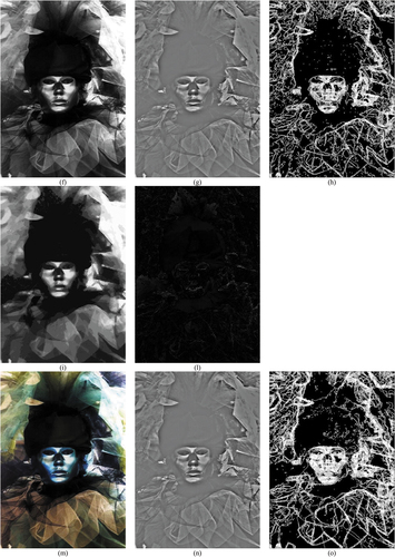
Figure 28. Continued.
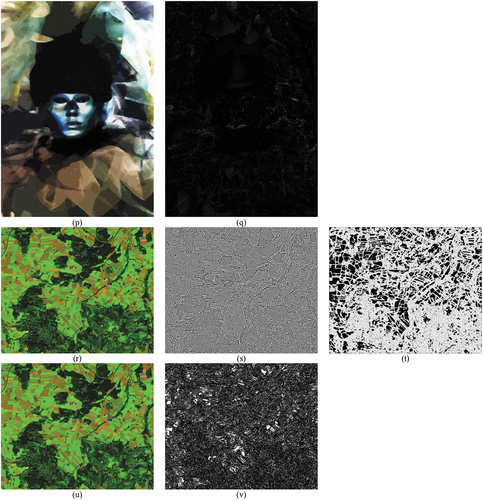
Figure 29. Adapted from (Griffin, Citation2006). Mathematically equivalent to a latent/hidden categorical variable (Baraldi, Citation2017; Baraldi & Tiede, Citation2018a, Citation2018b; Shotton et al., Citation2009; Wikipedia, Citation2015) (see ), color names are intuitive to think of and straightforward to display as color name-specific polyhedra in a color data space whose dimensionality ranges from 1 to 3. Central to this consideration is Berlin and Kay’s landmark study in linguistics of a “universal” inventory of eleven basic color (BC) words in twenty human languages (Berlin & Kay, Citation1969): black, white, gray, red, orange, yellow, green, blue, purple, pink and brown. Based on psychophysical evidence, human BC names can be mapped onto a monitor-typical RGB data cube as mutually exclusive and totally exhaustive polyhedra, neither necessarily convex nor connected (Griffin, Citation2006). Unlike RGB color naming polyhedralization of an RGB data cube, hypercolor naming hyperpolyhedralization of a multi-spectral (MS) reflectance hyperspace is difficult to think of and impossible to visualize when the number of MS channels is superior to three (Boynton, Citation1990), e.g., see .
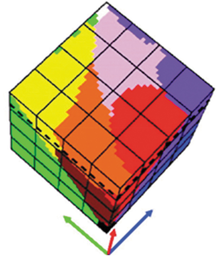
Figure 30. Unlike a 3-dimensional RGB true- or false-color data cube polyhedralization into RGB color names, which is intuitive to think of and straightforward to display (see ), a multi-spectral (MS) data space (hyper)polyhedralization into MS (hyper)color names is difficult to think of and impossible to visualize when the number of spectral channels is superior to three. As a possible example of hyperpolyhedron in a MS data hypercube, let us consider land cover (LC) class-specific (class-conditional) families of spectral signatures (Swain & Davis, Citation1978) in top-of-atmosphere reflectance (TOARF) values ∈ [0.0, 1.0], which include surface reflectance (SURF) values ∈ [0.0, 1.0] as a special case in clear sky and flat terrain conditions (Chavez, Citation1988), in agreement with EquationEquation (8)(8)
(8) to EquationEquation (11)
(11)
(11) . A within-class family of spectral signatures (e.g. dark-toned soil) in EquationEquation (8)
(8)
(8) = ‘TOARF ⊇ SURF’ values forms a buffer zone/ hyperpolyhedron/ envelope/ manifold/ joint distribution, depicted in light green, where SURF values as special case of TOARF values are depicted by a red line. Like a vector quantity has two characteristics, a magnitude and a direction, any LC class-specific MS manifold/hyperpolyhedron is characterized by a multivariate shape information component and a multivariate intensity information component. In the RS literature, typical prior knowledge-based spectral decision trees for MS data space partitioning (hyperpolyhedralization) into a finite and discrete vocabulary of MS color names, such as those adopted in the European Space Agency (ESA) Sentinel 2 (atmospheric, topographic and adjacency) Correction Prototype Processor (Sen2Cor) (DLR – Deutsches Zentrum für Luft-und Raumfahrt e.V. and VEGA Technologies, Citation2011; ESA – European Space Agency, Citation2015), the Multisensor Atmospheric Correction and Cloud Screening (MACCS)-Atmospheric/Topographic Correction (ATCOR) Joint Algorithm (MAJA) (Hagolle et al., Citation2017; Main-Knorn et al., Citation2018), the ATCOR commercial software toolbox (Richter & Schläpfer, Citation2012), the U.S. Geological Survey (USGS)-National Aeronautics and Space Administration (NASA) Landsat Ecosystem Disturbance Adaptive Processing System (LEDAPS) for Landsat-4/-5/-7 imagery (Vermote & Saleous, Citation2007) and the Landsat Surface Reflectance Code (LaSRC) for Landsat-8 imagery (Bilal et al., Citation2019; Qiu et al., Citation2019; USGS – U.S. Geological Survey, Citation2018b), typically adopt either a multivariate analysis of a stack of two-band spectral indexes or a logical (AND, OR) combination of univariate analyses (typically, scalar variable thresholding), where scalar spectral indexes or scalar spectral channels are analysed individually as univariate variables (Adamo et al., Citation2020; DLR – Deutsches Zentrum für Luft-und Raumfahrt e.V. and VEGA Technologies, Citation2011; ESA – European Space Agency, Citation2015; Gao, Citation1996; Goffi et al., Citation2020; Huth, Kuenzer, Wehrmann, Gebhardt, & Dech, Citation2012; Jordan, Citation1969; Kang Lee et al., Citation2018; Kashongwe et al., Citation2020; Key & Benson, Citation1999; Liang, Citation2004; Lozano et al., Citation2007; Marconcini et al., Citation2020; McFeeters, Citation1996; Neduni & Sivakumar, Citation2019; Rouse et al., Citation1974; Roy et al., Citation2009; Sykas, Citation2020; Tucker, Citation1979; Xu, Citation2006). A typical two-band spectral index is a scalar band ratio or band-pair difference equivalent to an angular coefficient (1st-order derivative) of a tangent to the spectral signature in one point, see and . It is well known that infinite functions can feature the same tangent value in one point. In practice, unlike combinations of basis functions working as universal approximators (Bishop, Citation1995; Cherkassky & Mulier, Citation1998), no combination of spectral indexes can reconstruct the multivariate shape and multivariate intensity information components of a spectral signature, see . As viable alternative to traditional static (non-adaptive to data) spectral rule-based decision trees for MS color naming found in the RS literature, based on thresholding either scalar spectral channels or scalar spectral indexes (Liang, Citation2004) (see ), such as the per-pixel decision tree implemented by the ESA Level 2 Sentinel-2 (atmospheric, adjacency and topographic) Correction Prototype Processor (Sen2Cor) software toolbox for Scene Classification Map (SCM) generation (DLR – Deutsches Zentrum für Luft-und Raumfahrt e.V. and VEGA Technologies, Citation2011; ESA – European Space Agency, Citation2015), the Satellite Image Automatic Mapper (SIAM)’s prior knowledge-based spectral decision tree (Baraldi, Citation2017, Citation2019a; Baraldi et al., Citation2010a, Citation2010b, Citation2018a, Citation2018b, Citation2006; Baraldi & Tiede, Citation2018a, Citation2018b) adopts a convergence-of-evidence approach to model any target family (ensemble) of spectral signatures, forming a hyperpolyhedron of interest in the MS reflectance hyperspace, as a combination of a multivariate shape information component with a multivariate intensity information component. For example, as shown above, typical spectral signatures of dark-toned soils and typical spectral signatures of light-toned soils form two MS envelopes in the MS reflectance hyperspace that approximately share the same multivariate shape information component, but whose pair of multivariate intensity information components does differ.
![Figure 30. Unlike a 3-dimensional RGB true- or false-color data cube polyhedralization into RGB color names, which is intuitive to think of and straightforward to display (see Figure 29), a multi-spectral (MS) data space (hyper)polyhedralization into MS (hyper)color names is difficult to think of and impossible to visualize when the number of spectral channels is superior to three. As a possible example of hyperpolyhedron in a MS data hypercube, let us consider land cover (LC) class-specific (class-conditional) families of spectral signatures (Swain & Davis, Citation1978) in top-of-atmosphere reflectance (TOARF) values ∈ [0.0, 1.0], which include surface reflectance (SURF) values ∈ [0.0, 1.0] as a special case in clear sky and flat terrain conditions (Chavez, Citation1988), in agreement with EquationEquation (8)(8) \lsquoDNs≥ 0atEOLevel0⊇TOARF∈0.0, 1.0atEOLevel1⊇SURF∈0.0, 1.0atEOLevel2/currentARD⊇Surfacealbedo∈0.0, 1.0at,say,EOLevel3/nextgenerationARD\rsquo(8)(8) to EquationEquation (11)(11) \lsquoTOARF≈SURF\rsquo(11) . A within-class family of spectral signatures (e.g. dark-toned soil) in EquationEquation (8)(8) \lsquoDNs≥ 0atEOLevel0⊇TOARF∈0.0, 1.0atEOLevel1⊇SURF∈0.0, 1.0atEOLevel2/currentARD⊇Surfacealbedo∈0.0, 1.0at,say,EOLevel3/nextgenerationARD\rsquo(8)(8) = ‘TOARF ⊇ SURF’ values forms a buffer zone/ hyperpolyhedron/ envelope/ manifold/ joint distribution, depicted in light green, where SURF values as special case of TOARF values are depicted by a red line. Like a vector quantity has two characteristics, a magnitude and a direction, any LC class-specific MS manifold/hyperpolyhedron is characterized by a multivariate shape information component and a multivariate intensity information component. In the RS literature, typical prior knowledge-based spectral decision trees for MS data space partitioning (hyperpolyhedralization) into a finite and discrete vocabulary of MS color names, such as those adopted in the European Space Agency (ESA) Sentinel 2 (atmospheric, topographic and adjacency) Correction Prototype Processor (Sen2Cor) (DLR – Deutsches Zentrum für Luft-und Raumfahrt e.V. and VEGA Technologies, Citation2011; ESA – European Space Agency, Citation2015), the Multisensor Atmospheric Correction and Cloud Screening (MACCS)-Atmospheric/Topographic Correction (ATCOR) Joint Algorithm (MAJA) (Hagolle et al., Citation2017; Main-Knorn et al., Citation2018), the ATCOR commercial software toolbox (Richter & Schläpfer, Citation2012), the U.S. Geological Survey (USGS)-National Aeronautics and Space Administration (NASA) Landsat Ecosystem Disturbance Adaptive Processing System (LEDAPS) for Landsat-4/-5/-7 imagery (Vermote & Saleous, Citation2007) and the Landsat Surface Reflectance Code (LaSRC) for Landsat-8 imagery (Bilal et al., Citation2019; Qiu et al., Citation2019; USGS – U.S. Geological Survey, Citation2018b), typically adopt either a multivariate analysis of a stack of two-band spectral indexes or a logical (AND, OR) combination of univariate analyses (typically, scalar variable thresholding), where scalar spectral indexes or scalar spectral channels are analysed individually as univariate variables (Adamo et al., Citation2020; DLR – Deutsches Zentrum für Luft-und Raumfahrt e.V. and VEGA Technologies, Citation2011; ESA – European Space Agency, Citation2015; Gao, Citation1996; Goffi et al., Citation2020; Huth, Kuenzer, Wehrmann, Gebhardt, & Dech, Citation2012; Jordan, Citation1969; Kang Lee et al., Citation2018; Kashongwe et al., Citation2020; Key & Benson, Citation1999; Liang, Citation2004; Lozano et al., Citation2007; Marconcini et al., Citation2020; McFeeters, Citation1996; Neduni & Sivakumar, Citation2019; Rouse et al., Citation1974; Roy et al., Citation2009; Sykas, Citation2020; Tucker, Citation1979; Xu, Citation2006). A typical two-band spectral index is a scalar band ratio or band-pair difference equivalent to an angular coefficient (1st-order derivative) of a tangent to the spectral signature in one point, see Figure 7 and Table 3. It is well known that infinite functions can feature the same tangent value in one point. In practice, unlike combinations of basis functions working as universal approximators (Bishop, Citation1995; Cherkassky & Mulier, Citation1998), no combination of spectral indexes can reconstruct the multivariate shape and multivariate intensity information components of a spectral signature, see Figure 7. As viable alternative to traditional static (non-adaptive to data) spectral rule-based decision trees for MS color naming found in the RS literature, based on thresholding either scalar spectral channels or scalar spectral indexes (Liang, Citation2004) (see Table 3), such as the per-pixel decision tree implemented by the ESA Level 2 Sentinel-2 (atmospheric, adjacency and topographic) Correction Prototype Processor (Sen2Cor) software toolbox for Scene Classification Map (SCM) generation (DLR – Deutsches Zentrum für Luft-und Raumfahrt e.V. and VEGA Technologies, Citation2011; ESA – European Space Agency, Citation2015), the Satellite Image Automatic Mapper (SIAM)’s prior knowledge-based spectral decision tree (Baraldi, Citation2017, Citation2019a; Baraldi et al., Citation2010a, Citation2010b, Citation2018a, Citation2018b, Citation2006; Baraldi & Tiede, Citation2018a, Citation2018b) adopts a convergence-of-evidence approach to model any target family (ensemble) of spectral signatures, forming a hyperpolyhedron of interest in the MS reflectance hyperspace, as a combination of a multivariate shape information component with a multivariate intensity information component. For example, as shown above, typical spectral signatures of dark-toned soils and typical spectral signatures of light-toned soils form two MS envelopes in the MS reflectance hyperspace that approximately share the same multivariate shape information component, but whose pair of multivariate intensity information components does differ.](/cms/asset/ff86034f-7965-45aa-9cf3-6623faa8a349/tbed_a_2017549_f0030_c.jpg)
Figure 31. One segmentation map is deterministically generated from one multi-level (e.g. binary) image, such as a thematic map, but the vice versa does not hold, i.e. many multi-level images can generate the same segmentation map. (a) To accomplish the deterministic task of segmentation map generation from a multi-level image, the two-pass connected-component multi-level image labeling algorithm (Dillencourt et al., Citation1992; Sonka et al., Citation1994) requires two raster scans of the input data set. In the figure above, as an example, nine image-objects/segments S1 to S9 can be detected in the 3-level thematic map shown at left. (b) Example of a 4-adjacency cross-aura map, shown at right, where 4-adjacency cross-aura values belong to range {0, 4}, generated in linear time from a multi-level image, such as a two-level image, shown at left. In addition to depicting image-object contours for qualitative visual assessment, these 4-adjacency contour values are suitable for shape index estimation, such as scale-invariant roundness (compactness and no holiness) in range [0.0, 1.0] (Baraldi, Citation2017; Baraldi & Soares, Citation2017).
![Figure 31. One segmentation map is deterministically generated from one multi-level (e.g. binary) image, such as a thematic map, but the vice versa does not hold, i.e. many multi-level images can generate the same segmentation map. (a) To accomplish the deterministic task of segmentation map generation from a multi-level image, the two-pass connected-component multi-level image labeling algorithm (Dillencourt et al., Citation1992; Sonka et al., Citation1994) requires two raster scans of the input data set. In the figure above, as an example, nine image-objects/segments S1 to S9 can be detected in the 3-level thematic map shown at left. (b) Example of a 4-adjacency cross-aura map, shown at right, where 4-adjacency cross-aura values belong to range {0, 4}, generated in linear time from a multi-level image, such as a two-level image, shown at left. In addition to depicting image-object contours for qualitative visual assessment, these 4-adjacency contour values are suitable for shape index estimation, such as scale-invariant roundness (compactness and no holiness) in range [0.0, 1.0] (Baraldi, Citation2017; Baraldi & Soares, Citation2017).](/cms/asset/3cbb87b8-2617-48f7-a0d6-9fe7edb7bccf/tbed_a_2017549_f0031_c.jpg)
Figure 32. Example of a binary relationship R: A ⇒ B ⊆ A × B from set A = VocabularyOfColorNames, where discrete and finite categorical color names (refer to Subsection 3.3.1) are equivalent to a semi-symbolic latent/hidden variable (see ) with cardinality |A| = a = ColorVocabularyCardinality = 11, to set B = LegendOfObjectClassNames, where a discrete and finite vocabulary of classes of real-world objects is equivalent to a symbolic variable (refer to Subsection 3.3.1) with cardinality |B| = b = ObjectClassLegendCardinality = 6, where A × B is the 2-fold Cartesian product between sets A and B. The Cartesian product of two sets A × B is a set whose elements are ordered pairs. The size of Cartesian product A × B is rows × columns = a × b. Set B = LegendOfObjectClassNames is superset-of the typical taxonomy of land cover (LC) classes adopted by the remote sensing (RS) community, such as the fully-nested two-stage Food and Agriculture Organization (FAO) Land Cover Classification System (LCCS) taxonomy (Di Gregorio & Jansen, Citation2000), see . “Correct” table entries (marked as ✓) must be: (i) selected by domain experts and (ii) community-agreed upon (Baraldi et al., Citation2018a, Citation2018b). Hence, this binary relationship pertains to the domain of prior knowledge, mandatory in CV systems to make the inherently ill-posed cognitive problem of scene-from-image reconstruction and understanding (Matsuyama & Hwang, Citation1990) better conditioned for numerical solution (Baraldi, Citation2017; Baraldi et al., Citation2018a, Citation2018b; Baraldi & Tiede, Citation2018a, Citation2018b; Bishop, Citation1995; Cherkassky & Mulier, Citation1998; Dubey et al., Citation2018). In more detail, this binary relationship is equivalent to top-down semantic knowledge transfer, from human experts to machine (Laurini & Thompson, Citation1992) (refer to Subsection 4.1), in agreement with the notion of knowledge engineering (refer to Section 2). Defined as a branch of the engineering meta-science (Couclelis, Citation2012), knowledge engineering (Laurini and Thompson, Citation1992; Sowa, Citation2000) is typically responsible of combining semantic information primitives to instantiate a conceptual/ mental/ perceptual model/ ontology(D ⊆ W, L), to be community agreed upon, where W is the (physical) domain of being in a physical world, L is a language adopted for the purpose of talking (communicating) about D, while D is a physical world-(sub)domain of interest (Sowa, Citation2000, p. 492), such that semantic relationhip 'D ⊆ W’ holds (refer to Section 2). Worth mentioning, a prior knowledge-based binary relationship between color names and target classes of real-world objects should never be confused with a bivariate frequency table (confusion matrix), pertaining to the domain of statistics (Baraldi, Citation2017; Baraldi et al., Citation2018a, Citation2018b; Baraldi & Tiede, Citation2018a, Citation2018b; Congalton & Green, Citation1999; Lunetta & Elvidge, Citation1999). Intuitively, in agreement with commonsense knowledge (Etzioni, Citation2017; Expert.ai, Citation2020; Thompson, Citation2018; U.S. DARPA – Defense Advanced Research Projects Agency, Citation2018; Wikipedia, Citation2021c) (refer to Section 2), on the one hand, the same color name can be shared by several classes of real world-objects. On the other hand, a single class of real-world objects can feature several color names as photometric attribute instantiation (Baraldi, Citation2017; Baraldi et al., Citation2018a, Citation2018b; Baraldi & Tiede, Citation2018a, Citation2018b). For example, Adams et al. correctly observed that discrete spectral end-members typically adopted in hyper-spectral image interpretation “cannot always be inverted to unique LC class names” (Adams et al., Citation1995).
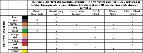
Table 3. Examples of scalar spectral indexes, implemented as either two-band or three-band functions, largely adopted by the remote sensing (RS) meta-science community in the feature engineering phase (Koehrsen, Citation2018), preliminary to (EO) optical image understanding (analysis, interpretation). Popular two-band spectral indexes are conceptually equivalent to the slope/ 1st-order derivative/ angular coefficient of a tangent to the spectral signature in one point (Baraldi, Citation2017, Citation2019a; Baraldi et al., Citation2010a, Citation2010b, Citation2018a, Citation2018b, Citation2006; Baraldi & Tiede, Citation2018a, Citation2018b; Liang, Citation2004), see . Each 1st-order derivative is typically considered useful in EO optical image understanding for the detection of one specific land cover (LC) class. Hence, the name of each two-band spectral index is typically proposed as LC class-specific. Unfortunately, it is well known that infinite functions (e.g. infinite spectral signatures) can feature the same 1st-order derivative in one point. In general, no combination of derivatives of any order can work as set of basis functions, capable of universal function approximation (Bishop, Citation1995; Cherkassky & Mulier, Citation1998). Lack of knowledge about these first principles has negative consequences on the RS common practice. First, the number and variety of scalar spectral index formulations proposed by the RS community to be considered better cross-correlated with their target LC class-specific family (envelope) of spectral signatures are ever increasing. Second, the number of scalar spectral indexes extracted from a multi-spectral (MS) signature tends to be equal or superior to the original dimensionality of the multi-spectral (MS) data space. It means that not only these scalar spectral indexes encode a lossy (irreversible) compression of a spectral signature, but their ensemble accomplishes no MS data compression at all, e.g. refer to works published in (Adamo et al., Citation2020; Goffi, Stroppiana, Brivio, Bordogna, & Boschetti, Citation2020; Kashongwe, Roy, & Bwangoy, Citation2020; Marconcini et al., Citation2020) as negative examples of MS feature engineering not to be imitated. Any increase in feature space dimensionality means increased secondary memory occupation, run-time memory occupation, computation time and cardinality of the training data set required by any machine learning (ML)-from-data algorithm to cope with the curse of data dimensionality (Bishop, Citation1995; Cherkassky & Mulier, Citation1998).
Figure 33. Phenological transitions in time: traditional driven-without-knowledge versus innovative driven-by-knowledge (stratified, masked, class-conditional) inductive data learning approach to either pixel-based or image object-based vegetation/not-vegetation classification through time, in a time series of, for example, 8-band WorldView-2 multi-spectral (MS) images. Traditional approach (Huth et al., Citation2012): Step (1) = Driven-without-knowledge vegetation spectral index extraction (see ) through time, either pixel-based or image object-based. In more detail, the well-known two-band Normalized Difference Vegetation Index (NDVI) (Jordan, Citation1969; Liang, Citation2004; Neduni & Sivakumar, Citation2019; Rouse et al., Citation1974; Sykas, Citation2020; Tucker, Citation1979) is employed, where NDVI ∈ [−1.0, 1.0] = f1(Red, NIR) = (NIR0.78÷0.90 – Red0.65÷0.68)/(NIR0.78÷0.90 + Red0.65÷0.68), which is monotonically increasing with the dimensionless Vegetation Ratio Index (VRI), where VRI ∈ (0, +∞) = NIR0.78÷0.90 / Red0.65÷0.68 = (1. + NDVI)/(1. – NDVI) (Liang, 2002), see . Hence, NDVI = f1(R, NIR) is conceptually equivalent to the angular coefficient (1st-order derivative) of a tangent to the spectral signature in one point (Baraldi, Citation2017, Citation2019a; Baraldi et al., Citation2010a, Citation2010b, Citation2018a, Citation2018b, Citation2006; Baraldi & Tiede, Citation2018a, Citation2018b; Liang, Citation2004). Step (2) = Pixel- or object-based supervised NDVI data classification, equivalent to posterior probability p(c = Vegetation class | NDVI = f1(R, NIR)), e.g. C5.0 supervised data learning decision tree classification (Huth et al., Citation2012). As viable alternative to the aforementioned step (1), for vegetation detection purposes, the traditional univariate two-band NDVI analysis through time is replaced by a more informative and more efficient class-conditional multi-variate data analysis of all spectral channels through time. In practice, automatic linear-time estimation of a class-conditional scalar greenness index (GI), p(GI = f9(R, NIR, MIR1) | Vegetation class = g(h(All Bands))), can be applied through time for within-vegetation class discrimination, based on: (i) a three-band scalar greenness index, GI, equivalent to a (downward) concavity (2nd-order derivative) centered on the NIR waveband = f9(R, NIR, MIR1) ∈ [0,∞) = max {0, (NIR/R) + (NIR/MIR1.55÷1.75) − (R/MIR1.55÷1.75)} ≥ 0 (Baraldi et al., Citation2010a) (see ), (ii) a Vegetation class, estimated (with approximation) by a logical-AND/OR combination of Satellite Image Automatic Mapper (SIAM)’s color names (see ), where each SIAM color name = h(All Bands) (Baraldi, Citation2017, Citation2019a; Baraldi et al., Citation2010a, Citation2010b, Citation2018a, Citation2018b, Citation2006; Baraldi & Tiede, Citation2018a, Citation2018b) (see ), hence, Vegetation class ≈ g(color names) = g(h(All Bands)), see .
![Figure 33. Phenological transitions in time: traditional driven-without-knowledge versus innovative driven-by-knowledge (stratified, masked, class-conditional) inductive data learning approach to either pixel-based or image object-based vegetation/not-vegetation classification through time, in a time series of, for example, 8-band WorldView-2 multi-spectral (MS) images. Traditional approach (Huth et al., Citation2012): Step (1) = Driven-without-knowledge vegetation spectral index extraction (see Figure 7) through time, either pixel-based or image object-based. In more detail, the well-known two-band Normalized Difference Vegetation Index (NDVI) (Jordan, Citation1969; Liang, Citation2004; Neduni & Sivakumar, Citation2019; Rouse et al., Citation1974; Sykas, Citation2020; Tucker, Citation1979) is employed, where NDVI ∈ [−1.0, 1.0] = f1(Red, NIR) = (NIR0.78÷0.90 – Red0.65÷0.68)/(NIR0.78÷0.90 + Red0.65÷0.68), which is monotonically increasing with the dimensionless Vegetation Ratio Index (VRI), where VRI ∈ (0, +∞) = NIR0.78÷0.90 / Red0.65÷0.68 = (1. + NDVI)/(1. – NDVI) (Liang, 2002), see Table 3. Hence, NDVI = f1(R, NIR) is conceptually equivalent to the angular coefficient (1st-order derivative) of a tangent to the spectral signature in one point (Baraldi, Citation2017, Citation2019a; Baraldi et al., Citation2010a, Citation2010b, Citation2018a, Citation2018b, Citation2006; Baraldi & Tiede, Citation2018a, Citation2018b; Liang, Citation2004). Step (2) = Pixel- or object-based supervised NDVI data classification, equivalent to posterior probability p(c = Vegetation class | NDVI = f1(R, NIR)), e.g. C5.0 supervised data learning decision tree classification (Huth et al., Citation2012). As viable alternative to the aforementioned step (1), for vegetation detection purposes, the traditional univariate two-band NDVI analysis through time is replaced by a more informative and more efficient class-conditional multi-variate data analysis of all spectral channels through time. In practice, automatic linear-time estimation of a class-conditional scalar greenness index (GI), p(GI = f9(R, NIR, MIR1) | Vegetation class = g(h(All Bands))), can be applied through time for within-vegetation class discrimination, based on: (i) a three-band scalar greenness index, GI, equivalent to a (downward) concavity (2nd-order derivative) centered on the NIR waveband = f9(R, NIR, MIR1) ∈ [0,∞) = max {0, (NIR/R) + (NIR/MIR1.55÷1.75) − (R/MIR1.55÷1.75)} ≥ 0 (Baraldi et al., Citation2010a) (see Table 3), (ii) a Vegetation class, estimated (with approximation) by a logical-AND/OR combination of Satellite Image Automatic Mapper (SIAM)’s color names (see Figure 32), where each SIAM color name = h(All Bands) (Baraldi, Citation2017, Citation2019a; Baraldi et al., Citation2010a, Citation2010b, Citation2018a, Citation2018b, Citation2006; Baraldi & Tiede, Citation2018a, Citation2018b) (see Figure 30), hence, Vegetation class ≈ g(color names) = g(h(All Bands)), see Figure 32.](/cms/asset/3052628c-565f-4248-a4af-c2e2e7b1a93f/tbed_a_2017549_f0033_c.jpg)
Figure 34. Six-stage (plus one, identified as stage zero) hybrid (combined deductive/ top-down/ prior knowledge-based and inductive/ bottom-up/ statistical model-based) feedback (provided with feedback loops) ‘CV ⊃ EO-IU ⊃ ARD’ system design (architecture), identified as QuickMap™ technology (refer to Section 2). In this figure, a rectangle with a different color fill is adopted to visualize each of the six stages for EO data processing (analysis, interpretation, understanding) plus stage zero for EO data pre-processing (data enhancement). Peculiar features of this original hybrid feedback ‘CV ⊃ EO-IU ⊃ ARD’ system design are summarized as follows. (i) It complies with the engineering principles of structured system design (Page-Jones, Citation1988), namely, modularity, hierarchy and regularity, considered neither necessary nor sufficient, but highly recommended for system scalability (Lipson, Citation2007). (ii) It complies with a convergence of spatial with color evidence approach to the cognitive task of vision, where spatial information typically dominates colorimetric information (Baraldi, Citation2017; Baraldi, Humber, Tiede, & Lang, Citation2018a; Baraldi, Humber, Tiede, & Lang, Citation2018b; Baraldi & Tiede, Citation2018a; Baraldi & Tiede, Citation2018b), see . In more detail, it is consistent with a well-known naïve Bayesian classification paradigm (Bishop, Citation1995; Cherkassky & Mulier, Citation1998), formulated as Equation (12), which is our original formulation of the adopted convergence-of-evidence approach. (iii) According to Bayesian constraints, it is required to: (a) accomplish retinotopic (spatial topology-preserving) 2D analysis of (2D) imagery (Baraldi, Citation2017; Baraldi & Alpaydin, Citation2002a; Baraldi & Alpaydin, Citation2002b; Fritzke, Citation1997; Martinetz, Berkovich, & Schulten, Citation1994; Öğmen & Herzog, Citation2010; Tsotsos, Citation1990) (see and ), (b) comply with the Mach bands visual illusion (Pessoa, Citation1996) (see ), etc. (refer to the body of Subsection 4.2). (iv) It is alternative to inductive feedforward ‘CV ⊃ EO-IU ⊃ ARD’ system architectures adopted by the RS mainstream, including inductive Deep Convolutional Neural Networks (DCNNs), learned from data end-to-end (Cimpoi, Maji, Kokkinos & Vedaldi, Citation2014; Krizhevsky, Sutskever, & Hinton, Citation2012). Worth noting, in the proposed six-stage hybrid feedback CV system design, relationship ‘Deductive (physical model-based, “hand-crafted”) DCNN → Hybrid feedback CV’ holds; it means that a deductive multi-scale multi-orientation DCNN (see ) is included (as part-of, without inheritance) in the proposed CV system. Hence, the proposed hybrid feedback CV system outpaces the “complexity” of traditional deductive or inductive feedforward DCNNs. For more details about the individual stages of the proposed six-stage hybrid feedback ‘CV ⊃ EO-IU ⊃ ARD’ system architecture, refer to the body text.
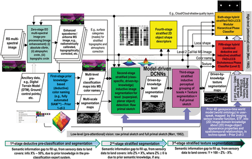
Figure 35. Comparison of existing EO sensory data-derived Level 2/Analysis Ready Data (ARD) information products, where dimensionless digital numbers (DNs ≥ 0) at Level 0 have been radiometrically corrected (calibrated) into top-of-atmosphere reflectance (TOARF) values in range [0.0, 1.0] at Level 1, whereas TOARF values at Level 1 are corrected from atmospheric and, eventually, topographic and adjacency effects into surface reflectance (SURF) values, belonging to range [0.0, 1.0], at Level 2 (Egorov, Roy, Zhang, Hansen, and Kommareddy, Citation2018). Adopted acronyms: Committee on Earth Observation Satellites (CEOS) ARD for Land (CARD4L) product definition (CEOS – Committee on Earth Observation Satellites, Citation2018); U.S. Geological Survey (USGS)-National Aeronautics and Space Administration (NASA) Landsat Ecosystem Disturbance Adaptive Processing System (LEDAPS) software executable for Landsat-4/-5/-7 imagery (Vermote & Saleous, Citation2007), plus Landsat Surface Reflectance Code (LaSRC) software executable for Landsat-8 imagery (Bilal et al., Citation2019; Qiu et al., Citation2019; USGS – U.S. Geological Survey, Citation2018b); Italian Space Agency (ASI) Hyperspectral Precursor and Application Mission (PRISMA) imaging sensor (ASI – Agenzia Spaziale Italiana, Citation2020; OHB, Citation2016); European Space Agency (ESA) EO Sentinel-2 data-derived Level 2 product, generated by the Sentinel 2 (atmospheric, topographic and adjacency) Correction Prototype Processor (Sen2Cor) (DLR – Deutsches Zentrum für Luft-und Raumfahrt e.V. and VEGA Technologies, Citation2011; ESA – European Space Agency, Citation2015). More acronyms adopted in this table: Digital Elevation Model (DEM), open source C Function of Mask (CFMask) algorithm (USGS – U.S. Geological Survey, Citation2018a, Citation2018c).
![Figure 35. Comparison of existing EO sensory data-derived Level 2/Analysis Ready Data (ARD) information products, where dimensionless digital numbers (DNs ≥ 0) at Level 0 have been radiometrically corrected (calibrated) into top-of-atmosphere reflectance (TOARF) values in range [0.0, 1.0] at Level 1, whereas TOARF values at Level 1 are corrected from atmospheric and, eventually, topographic and adjacency effects into surface reflectance (SURF) values, belonging to range [0.0, 1.0], at Level 2 (Egorov, Roy, Zhang, Hansen, and Kommareddy, Citation2018). Adopted acronyms: Committee on Earth Observation Satellites (CEOS) ARD for Land (CARD4L) product definition (CEOS – Committee on Earth Observation Satellites, Citation2018); U.S. Geological Survey (USGS)-National Aeronautics and Space Administration (NASA) Landsat Ecosystem Disturbance Adaptive Processing System (LEDAPS) software executable for Landsat-4/-5/-7 imagery (Vermote & Saleous, Citation2007), plus Landsat Surface Reflectance Code (LaSRC) software executable for Landsat-8 imagery (Bilal et al., Citation2019; Qiu et al., Citation2019; USGS – U.S. Geological Survey, Citation2018b); Italian Space Agency (ASI) Hyperspectral Precursor and Application Mission (PRISMA) imaging sensor (ASI – Agenzia Spaziale Italiana, Citation2020; OHB, Citation2016); European Space Agency (ESA) EO Sentinel-2 data-derived Level 2 product, generated by the Sentinel 2 (atmospheric, topographic and adjacency) Correction Prototype Processor (Sen2Cor) (DLR – Deutsches Zentrum für Luft-und Raumfahrt e.V. and VEGA Technologies, Citation2011; ESA – European Space Agency, Citation2015). More acronyms adopted in this table: Digital Elevation Model (DEM), open source C Function of Mask (CFMask) algorithm (USGS – U.S. Geological Survey, Citation2018a, Citation2018c).](/cms/asset/b433e9cb-7494-41d1-8bd9-accc02c0fe26/tbed_a_2017549_f0035_c.jpg)
Figure 36. Comparison of the CEOS ARD for Land Optical Surface Reflectance (CARD4L-OSR) product definition (CEOS – Committee on Earth Observation Satellites, Citation2018), supported by no computer vision (CV) software implementation, with existing ARD product implementations, namely, USGS-NASA ARD, ESA EO Level 2 and ASI PRISMA Level 1 and Level 2, also refer to .
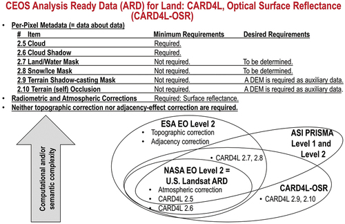
Figure 37. Non-standard general-purpose, user- and application-independent European Space Agency (ESA) Earth observation (EO) Level 2 Scene Classification Map (SCM) legend adopted by the sensor-specific Sentinel 2 (atmospheric, adjacency and topographic) Correction (Sen2Cor) Prototype Processor (DLR – Deutsches Zentrum für Luft-und Raumfahrt e.V. and VEGA Technologies, Citation2011; ESA – European Space Agency, Citation2015), developed, run and/or distributed free-of-cost by ESA to be run on the user side. Noteworthy, the ESA Sen2Core SCM’s LC class taxonomy does not comply with a standard Food and Agriculture Organization (FAO) of the United Nations (UN) Land Cover Classification System (LCCS) taxonomy, which is fully nested and whose first-stage 3-level 8-class FAO LCCS Dichotomous Phase (DP) taxonomy is general-purpose, user- and application-independent, see . This Sen2Cor’s SCM taxonomy is also alternative to the Cloud versus Not-Cloud (Rest-of-the-world) taxonomy proposed in the technical note “Harmonization of Cloud Classes” issued by the Copernicus Data Quality Control team (ESA – European Space Agency, Citation2017a) (refer to Section 2).
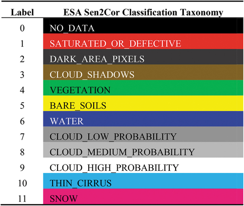
Figure 38. Sensor-specific Sentinel 2 (atmospheric, adjacency and topographic) Correction (Sen2Cor) Prototype Processor (DLR – Deutsches Zentrum für Luft-und Raumfahrt e.V. and VEGA Technologies, Citation2011; ESA – European Space Agency, Citation2015), developed and distributed free-of-cost by ESA to be run on the user side. The Sen2Cor flow chart for ESA Level 2 product generation from Sentinel-2 imagery (DLR – Deutsches Zentrum für Luft-und Raumfahrt e.V. and VEGA Technologies, Citation2011; ESA – European Space Agency, Citation2015) is the same as that in the Atmospheric/Topographic Correction for Satellite Imagery (ATCOR) commercial software toolbox (Richter & Schläpfer, Citation2012). While sharing the same system design, ESA Sen2Cor and ATCOR differ at the two lowest levels of system abstraction, namely, algorithm and implementation (Marr, Citation1982) (refer to Subsection 3.2). First, a Scene Classification Map (SCM) is generated from top-of-atmosphere reflectance (TOARF) values. Next, class-conditional MS image radiometric enhancement of TOARF into surface reflectance (SURF) 3-of-3 values (refer to Subsection 3.3.2), synonym for bottom-of-atmosphere (BOA) reflectance values, corrected for atmospheric effects (into SURF 1-of-3 values), topographic effects (into SURF 2-of-3 values) and adjacency effects (into SURF 3-of-3 values), is accomplished in sequence (Egorov, Roy, Zhang, Hansen, and Kommareddy, Citation2018), stratified/ layered/ masked by the same SCM product generated at first stage from TOARF values. More acronyms in this figure: AOT = aerosol optical thickness, DEM = digital elevation model, LUT = look-up table. Noteworthy, in the ESA Sen2Cor software workflow, the output SCM co-product and the output MS image co-product are not “aligned” with each other. Whereas the output SCM co-product is generated from EO Level 1 data in TOARF values, the output MS image consists of Level 2 data in SURF 3-of-3 values, whose radiometric quality is better (in terms of robustness) than that of TOARF values available at Level 1. Hence, the output Level 2 MS image in SURF 3-of-3 values is eligible for better interpretation (classification), which would deliver as output a new Level 2 SURF 3-of-3 data-derived SCM co-product, whose symbolic mapping is “aligned” with the Level 2 data in SURF 3-of-3 values and whose semantic quality (in terms of semantic depth and/or semantic accuracy) is expected to be better than that of the Level 1 TOARF data-derived SCM actually provided as Level 2 output symbolic co-product.
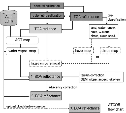
Figure 39. Semantics-enabled EO big raster-based (numerical) data and vector-based categorical (either subsymbolic, semi-symbolic or symbolic) information cube (Augustin et al., Citation2018, Citation2019; Baraldi et al., Citation2016, Citation2017; FFG – Austrian Research Promotion Agency, Citation2015, Citation2016, Citation2018, Citation2020; Sudmanns et al., Citation2021; Sudmanns et al., Citation2018; Tiede et al., Citation2017), synonym for artificial general intelligence (AGI) (Bills, Citation2020; Chollet, Citation2019; Dreyfus, Citation1965, Citation1991, Citation1992; EC – European Commission, Citation2019; Fjelland, Citation2020; Hassabis et al., Citation2017; Ideami, Citation2021; Jajal, Citation2018; Jordan, Citation2018; Mindfire Foundation, Citation2018; Practical AI, Citation2020; Romero, Citation2021; Santoro et al., Citation2021; Sweeney, Citation2018a; Wolski, Citation2020a, Citation2020b) for Data and Information Access Services (AGI4DIAS) = EquationEquation (1)(1)
(1) (see ), considered necessary-but-not-sufficient precondition to semantic content-based image retrieval (SCBIR) and semantics-enabled information/knowledge discovery (SEIKD) over heterogeneous data sources acquired through geospace-time and imaging sensors, where SCBIR and SEIKD are consistent with symbolic human reasoning in human-speak (Augustin et al., Citation2018, Citation2019; Baraldi, Citation2017; Baraldi & Tiede, Citation2018a, Citation2018b; Baraldi et al., Citation2016, Citation2017; Dhurba & King, Citation2005; Newell & Simon, Citation1972; Planet, Citation2018; Sudmanns et al., Citation2021; Sudmanns et al., Citation2018; Tiede et al., Citation2017), also refer to and . When stored in the multi-source EO image database, any EO Level 0 image in dimensionless digital numbers (DNs), provided with no physical meaning, is automatically transformed by default into, first, a sensory-data derived single-date EO Level 1 image, radiometrically calibrated into top-of-atmosphere reflectance (TOARF) values. Next, it is automatically transformed by an ‘AGI ⊃ CV ⊃ EO-IU ⊃ ARD’ system in operational mode into an innovative semantics-enriched ARD co-product pair comprising: (i) a single-date multi-spectral (MS) image, radiometrically calibrated from TOARF into surface reflectance (SURF) values, corrected for atmospheric, adjacency and topographic effects, stacked with: (ii) its EO data-derived value-adding Scene Classification Map (SCM), equivalent to a sensory image-derived categorical/ nominal/ qualitative variable of semantic quality, where the thematic map legend, comprising quality layers such as Cloud and Cloud–shadow, is general-purpose, user- and application-independent. In practice, an SCM is an instantiation of one of the Essential Climate Variables (ECVs) defined by the World Climate Organization (WCO) for the terrestrial layer (Bojinski et al., Citation2014), namely, land cover (including vegetation types) (see ), where ECVs are the EO data-derived value-adding information variables considered at the basis of the Information level in the Data-Information-Knowledge-Wisdom (DIKW) hierarchical conceptualization (Rowley, Citation2007; Rowley & Hartley, Citation2008; Wikipedia, Citation2020a; Zeleny, Citation1987, Citation2005; Zins, Citation2007) (see ) adopted by the GEO second implementation plan for years 2016–2025 of a Global Earth Observation System of (component) Systems (GEOSS) (GEO – Group on Earth Observations, Citation2015; Nativi et al., Citation2015, Citation2020; Santoro et al., Citation2017), see . As a possible augmentation, this innovative semantics-enriched ARD co-product pair can be stacked with (iii) EO data-derived value-adding numerical variables, either: (I) biophysical variables, e.g. leaf area index (LAI) (Liang, Citation2004), aboveground biomass, etc., belonging to the set of ECVs defined by the WCO (Bojinski et al., Citation2014) (see ), (II) class-conditional spectral indexes, e.g. vegetation class-conditional greenness index (Baraldi et al., Citation2010a, Citation2010b), and/or (III) categorical variables of subsymbolic quality (geographic field-objects) (Couclelis, Citation2010; Goodchild et al., Citation2007), e.g. fuzzy sets/discretization levels of a geographic field, such as fuzzy sets (Zadeh, Citation1965) low/ medium/ high of a numerical variable estimating speed, whether uncalibrated (dimensionless) or calibrated (provided with a physical unit of measure, say, km/h), etc. (Baraldi, Citation2017; Baraldi & Tiede, Citation2018a, Citation2018b). Unlike the proposed semantics-enabled EO big raster-based (numerical) data and vector-based (categorical) information cube management system, synonym for AGI4DIAS (see ), whose future developments depend on a more severe (more ambitious), but realistic multi-sensor EO optical sensory image-derived ARD co-product pair definition and software implementation to be community-agreed upon, existing operational country-wide EO (raster-based) data cubes, such as the Digital Earth Africa, Digital Earth Australia (Lewis et al., Citation2017), Swiss Data Cube (Giuliani et al., Citation2017), etc. (Giuliani et al., Citation2020), adopt the CEOS ARD for Land Optical Surface Reflectance (CARD4L-OSR) product definition as standard baseline (CEOS – Committee on Earth Observation Satellites, Citation2018) (see ), where an SCM is lacking as ARD symbolic co-product. As a consequence, they are affected by the data-rich information-poor (DRIP) syndrome (Ball, Citation2021; Bernus & Noran, Citation2017). In contrast with existing EO (raster-based) data cubes, systematic availability of an ARD symbolic co-product, namely, a sensory image-derived SCM co-product, is considered mandatory by a future generation of semantics-enabled EO raster-based data and vector-based information cube management systems (Augustin et al., Citation2018, Citation2019; Baraldi et al., Citation2017; FFG – Austrian Research Promotion Agency, Citation2015, Citation2016, Citation2018, Citation2020; Sudmanns et al., Citation2018; Tiede et al., Citation2017), synonym for AGI4DIAS = EquationEquation (1)
(1)
(1) , see .
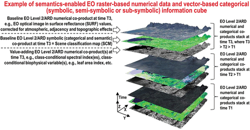
Figure 40. Architecture (design) of a closed-loop artificial general intelligence (AGI) (Bills, Citation2020; Chollet, Citation2019; Dreyfus, Citation1965, Citation1991, Citation1992; EC – European Commission, Citation2019; Fjelland, Citation2020; Hassabis et al., Citation2017; Ideami, Citation2021; Jajal, Citation2018; Jordan, Citation2018; Mindfire Foundation, Citation2018; Practical AI, Citation2020; Romero, Citation2021; Santoro et al., Citation2021; Sweeney, Citation2018a; Wolski, Citation2020a, Citation2020b) for Data and Information Access Services (AGI4DIAS) = EquationEquation (1)(1)
(1) , synonym for semantics-enabled EO big raster-based (numerical) data and vector-based categorical (either subsymbolic, semi-symbolic or symbolic) information cube management system (Augustin et al., Citation2018, Citation2019; Baraldi et al., Citation2016, Citation2017; FFG – Austrian Research Promotion Agency, Citation2015, Citation2016, Citation2018, Citation2020; Sudmanns et al., Citation2021; Sudmanns et al., Citation2018; Tiede et al., Citation2017) (see ), capable of incremental (semantic) learning. AGI4DIAS is considered necessary-but-not-sufficient precondition to semantic content-based image retrieval (SCBIR) and semantics-enabled information/knowledge discovery (SEIKD) over heterogeneous data sources acquired through geospace-time and imaging sensors, where SCBIR and SEIKD are consistent with symbolic human reasoning in human-speak (Augustin et al., Citation2018, Citation2019; Baraldi, Citation2017; Baraldi & Tiede, Citation2018a, Citation2018b; Baraldi et al., Citation2016, Citation2017; Dhurba & King, Citation2005; Newell & Simon, Citation1972; Planet, Citation2018; Sudmanns et al., Citation2021; Sudmanns et al., Citation2018; Tiede et al., Citation2017), also refer to and . The AGI4DIAS system architecture (design) consists of a feedback hybrid ‘ARD ⊂ EO-IU ⊂ CV ⊂ AGI’ = EquationEquation (3)
(3)
(3) subsystem (see ) in closed-loop with an EO Semantic Querying (SQ) subsystem. The hybrid feedback ‘ARD ⊂ EO-IU ⊂ CV ⊂ AGI’ = EquationEquation (3)
(3)
(3) component system (see ) is required to be in operational mode, automatic (no human-machine interaction is required by the EO-IU subsystem to run) and near real-time, to provide the EO-SQ subsystem with value-adding EO sensory data-derived information products, including a Scene Classification Map (SCM), considered necessary-but-not-sufficient pre-condition to SQ, encompassing SCBIR and SEIKD operations in massive multi-source EO image bases. The EO-SQ subsystem is provided with a graphic user interface (GUI), to streamline: (i) top-down knowledge transfer, from-human-to-machine, of an a priori conceptual (mental) model of the 4D spatial-temporal real-world, (ii) high-level user- and application-specific SCBIR and SEIKD queries. Output products generated by the closed-loop AGI4DIAS system are expected to monotonically increase their value-added informativeness with closed-loop iterations, according to Bayesian updating, where Bayesian inference is applied iteratively: after observing some evidence, the resulting posterior probability can be treated as a prior probability and a new posterior probability computed from new evidence (Bowers & Davis, Citation2012; Ghahramani, Citation2011; Lähteenlahti, Citation2021; Sarkar, Citation2018).
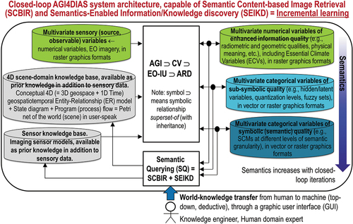
Figure 41. In agreement with symbols adopted by the standard Unified Modeling Language (UML) for graphical modeling of object-oriented software (Fowler, Citation2003), relationship part-of, denoted with symbol ‘→’ pointing from the supplier to the client, should not to be confused with relationship subset-of, ‘⊃’, meaning specialization with inheritance from the superset (at left) to the subset. A National Aeronautics and Space Administration (NASA) EO (e.g. Landsat-8) Level 2 product is defined as “a data-derived geophysical variable at the same resolution and location as Level 1 source data” (NASA, Citation2018). Herein, subsymbolic NASA EO Level 2 is considered part-of a semantics-enriched ESA EO (e.g. Sentinel-2) sensory image-derived Level 2/Analysis Ready Data (ARD) co-product pair, defined as (DLR – Deutsches Zentrum für Luft-und Raumfahrt e.V. and VEGA Technologies, Citation2011; ESA – European Space Agency, Citation2015): (a) a single-date multi-spectral (MS) image whose digital numbers (DNs) are radiometrically calibrated into surface reflectance (SURF) 3-of-3 values (refer to Subsection 3.3.2), corrected in sequence for atmospheric effects (into SURF 1-of-3 values), topographic effects (into SURF 2-of-3 values) and adjacency effects (into SURF 3-of-3 values) (Egorov, Roy, Zhang, Hansen, and Kommareddy, Citation2018), stacked with (b) its data-derived general-purpose, user- and application-independent Scene Classification Map (SCM), whose thematic map legend includes quality layers Cloud and Cloud–shadow. A semantics-enriched ESA EO Level 2 co-product pair is regarded as an information primitive (unit of information) to be accomplished by Artificial General Intelligence for the Space segment (AGI4Space), such as in future intelligent small satellite constellations (EOportal, Citation2020; ESA – European Space Agency, Citation2019; Esposito et al., Citation2019a, Citation2019b; GISCafe News, Citation2018; Zhou, Citation2001), and/or at the midstream segment in an AGI for Data and Information Access Services (AGI4DIAS) framework, see . In the graphical representation shown above, additional acronyms of interest are computer vision (CV), whose special case is EO image understanding (EO-IU) in operational mode, semantic content-based image retrieval (SCBIR), semantics-enabled information/knowledge discovery (SEIKD), where SCBIR + SEIKD is considered synonym for AGI4DIAS (see ), and Global Earth Observation System of (component) Systems (GEOSS), defined by the Group on Earth Observations (GEO) (EC – European Commission and GEO – Group on Earth Observations, Citation2014; GEO – Group on Earth Observations, Citation2005, Citation2019; Mavridis, Citation2011) and revised by GEO for years 2016–2025 as a new expert EO data-derived information and knowledge system (GEO – Group on Earth Observations, Citation2015; Nativi et al., Citation2015, Citation2020; Santoro et al., Citation2017), see . Proposed in (Baraldi, Citation2017; Baraldi & Tiede, Citation2018a, Citation2018b), this working hypothesis postulates that GEOSS, whose parts-of are the still-unsolved (open) problems of SCBIR and SEIKD, cannot be achieved until the necessary-but-not-sufficient precondition of CV in operational mode, specifically, systematic semantics-enriched ESA-like EO image-derived Level 2 co-product pair generation, is accomplished in advance. If the aforementioned working hypothesis holds true, then the complexity of SCBIR and SEIKD is not inferior to the complexity of vision, acknowledged to be inherently ill-posed in the Hadamard sense (Hadamard, Citation1902) and non-deterministic polynomial (NP)-hard in computational complexity (Baraldi, Citation2017; Baraldi et al., Citation2018a, Citation2018b; Baraldi & Tiede, Citation2018a, Citation2018b; Frintrop, Citation2011; Matsuyama & Hwang, Citation1990; Tsotsos, Citation1990), see . In other words, SCBIR, SEIKD and CV are all AGI-complete problems (Saba, Citation2020c; Wikipedia, Citation2021a) (refer to Section2). To make the inherently-ill-posed CV problem better conditioned for numerical solution (Baraldi, Citation2017; Bishop, Citation1995; Cherkassky & Mulier, Citation1998; Dubey et al., Citation2018), a CV system is constrained to include (as part-of) a computational model of human vision (Baraldi, Citation2017; Baraldi et al., Citation2018a, Citation2018b; Baraldi & Tiede, Citation2018a, Citation2018b; Iqbal & Aggarwal, Citation2001), i.e. EquationEquation (4)(4)
(4) = ‘Human vision → CV’ holds (see ), in agreement with a reverse engineering approach to CV (Bharath & Petrou, Citation2008; DiCarlo, Citation2017), see .
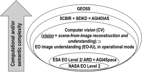
Figure 42. Example of automatic SIAM-based post-classification MS color naming change/no-change detection, starting from MS images acquired from different EO imaging sensors harmonized at the SIAM categorical level of color naming (see and ), where SIAM stays for Satellite Image Automatic Mapper (SIAM) (Baraldi, Citation2017, Citation2019a; Baraldi et al., Citation2006, Citation2010a, Citation2010b, Citation2018a, Citation2018b; Baraldi & Tiede, Citation2018a, Citation2018b). Left: SIAM map depicted in 33 pseudo-colors, generated from a SPOT-5 image featuring four channels, specifically, visible green (G), visible red (R), near infrared (NIR) and middle infrared (MIR), radiometrically calibrated into TOARF values, upscaled to 5 m resolution. Center: SIAM map depicted in 33 pseudo-colors, generated from a RapidEye image featuring four channels, specifically, visible blue (B), G, R and NIR, radiometrically calibrated into TOARF values, 5 m resolution. Left: Multi-source SIAM-based post-classification change/no-change detection map, whose map legend consists of 29 codewords, depicted in pseudo-colors and associated with cells in a two-way 33 × 33 transition matrix with 33 entries as color names per date. The bi-temporal SIAM-based post-classification map legend is shown in and .
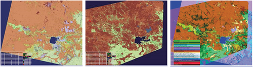
Figure 43. Prior knowledge-based/ top-down/ deductive two-way transition matrix, implemented for a bi-temporal pair of SIAM maps generated at time T1 (rows) < time T2 (columns), such as that shown in , featuring the same so-called “shared” (across-sensor) vocabulary (legend) of 33 color names, which guarantess semantic/ontological interoperability of SIAM maps generated from different “families” of EO optical imaging sensors, see Table 4 in the Part 2 (Baraldi et al., Citation2022) of this two-part paper. This prior knowledge-based bi-temporal SIAM-based post-classification change/no-change transition matrix is yet-another example of top-down semantic knowledge transfer, from human experts to machine (Laurini & Thompson, Citation1992), to be considered mandatory by inherently ill-posed programmable data-crunching machine (computers), whose being is not in-the-world of humans (Dreyfus, Citation1965, Citation1991, Citation1992) (refer to Section 2), to become better posed (conditioned) for numerical and/or symbolic solution (refer to Subsection 4.1). This top-down/deductive two-way transition matrix provides as output a discrete and finite categorical variable, generated from the combination through time of the two input categorical variables. Specifically, the output categorical variable is a bi-temporal SIAM-based post-classification change/no-change map legend, shown in . In the output symbolic (categorical and semantic) map legend, semantics-through-time (specifically, bi-temporal semantics) is superior to semantics of the single-date symbolic (categorical and semantic) map legend shared by the two input single-date symbolic or semi-symbolic maps (refer to Subsection 3.3.1). In other words, in general, meaning/semantics increases through time. In the RS common practice, as viable alternative to numerical data time-series analysis, post-classification LC change/no-change (LCCNC) analysis (detection, tracking-through-time) is recommended for its (symbolic) simplicity and (computational) efficiency if and only if single-date overall accuracy (OA) values are (fuzzy, qualitatively) “high” through the thematic map time-series (Baraldi, Citation2017; Baraldi et al., Citation2018a, Citation2018b), see EquationEquation (15)(15)
(15) . Moreover, even when a time-series of single-date semantic maps is considered accurate, how should a bi-temporal semantic transition matrix, such as that shown in Figure 43, deal with transitions in semantics which are possible in theory, but are considered either unlikely in the real-world, say, from LC class Snow at time T1 to LC class Active Fire at time T2 > time T1, or are affected by “semantic noise”, say, from LC class Vegetation at time T1 to class Cloud at time T2 > time T1? These practical cases in “noisy” semantic transitions through time must be modeled top-down by a human domain-expert to be coped with accordingly by the machine, whose being is not in the world of humans (Dreyfus, Citation1965, Citation1991, Citation1992) (refer to Section 2), see how “noisy” semantic transitions are modeled top-down in the present Figure 43 in combination with .
![Figure 43. Prior knowledge-based/ top-down/ deductive two-way transition matrix, implemented for a bi-temporal pair of SIAM maps generated at time T1 (rows) < time T2 (columns), such as that shown in Figure 42, featuring the same so-called “shared” (across-sensor) vocabulary (legend) of 33 color names, which guarantess semantic/ontological interoperability of SIAM maps generated from different “families” of EO optical imaging sensors, see Table 4 in the Part 2 (Baraldi et al., Citation2022) of this two-part paper. This prior knowledge-based bi-temporal SIAM-based post-classification change/no-change transition matrix is yet-another example of top-down semantic knowledge transfer, from human experts to machine (Laurini & Thompson, Citation1992), to be considered mandatory by inherently ill-posed programmable data-crunching machine (computers), whose being is not in-the-world of humans (Dreyfus, Citation1965, Citation1991, Citation1992) (refer to Section 2), to become better posed (conditioned) for numerical and/or symbolic solution (refer to Subsection 4.1). This top-down/deductive two-way transition matrix provides as output a discrete and finite categorical variable, generated from the combination through time of the two input categorical variables. Specifically, the output categorical variable is a bi-temporal SIAM-based post-classification change/no-change map legend, shown in Figure 44. In the output symbolic (categorical and semantic) map legend, semantics-through-time (specifically, bi-temporal semantics) is superior to semantics of the single-date symbolic (categorical and semantic) map legend shared by the two input single-date symbolic or semi-symbolic maps (refer to Subsection 3.3.1). In other words, in general, meaning/semantics increases through time. In the RS common practice, as viable alternative to numerical data time-series analysis, post-classification LC change/no-change (LCCNC) analysis (detection, tracking-through-time) is recommended for its (symbolic) simplicity and (computational) efficiency if and only if single-date overall accuracy (OA) values are (fuzzy, qualitatively) “high” through the thematic map time-series (Baraldi, Citation2017; Baraldi et al., Citation2018a, Citation2018b), see EquationEquation (15)(15) x0026;Bi0temporal post0classification LC change/no0change (LCCNC) x0026;detection overall accuracy (OA),OA0LCCNC1,2∈[0, 1],where OA0LCCNC1,2=x0026;f(independent variables OA of the LC map at time T1,identified as OA0LC1,x0026;and OA of the LC map at time T2,identified as OA-LC2, with T1T2)=x0026;f(OA0LC1,OA0LC2)≤OA0LC1×OA0LC2,x0026; where OA0LC1∈[0,1] and OA0LC2∈[0, 1].(15) . Moreover, even when a time-series of single-date semantic maps is considered accurate, how should a bi-temporal semantic transition matrix, such as that shown in Figure 43, deal with transitions in semantics which are possible in theory, but are considered either unlikely in the real-world, say, from LC class Snow at time T1 to LC class Active Fire at time T2 > time T1, or are affected by “semantic noise”, say, from LC class Vegetation at time T1 to class Cloud at time T2 > time T1? These practical cases in “noisy” semantic transitions through time must be modeled top-down by a human domain-expert to be coped with accordingly by the machine, whose being is not in the world of humans (Dreyfus, Citation1965, Citation1991, Citation1992) (refer to Section 2), see how “noisy” semantic transitions are modeled top-down in the present Figure 43 in combination with Figure 44.](/cms/asset/8dad55d2-0a18-4718-a5bd-c56cbddcdf00/tbed_a_2017549_f0043_c.jpg)
Figure 44. Bi-temporal SIAM-based post-classification change/no-change map legend, consisting of 29 change/no-change bi-temporal MS color name combinations, depicted with pseudo-colors, identified by a two-way 33 × 33 transition matrix featuring 33 entries as color names per date, see . This prior knowledge-based bi-temporal SIAM-based post-classification change/no-change map legend is yet-another example of top-down semantic knowledge transfer, from human experts to machine (Laurini & Thompson, Citation1992), to be considered mandatory by inherently ill-posed programmable data-crunching machine (computers), that are not in-the-world (Dreyfus, Citation1965, Citation1991, Citation1992) (refer to Section 2), to become better posed (conditioned) for numerical and/or symbolic solution (refer to Subsection 4.1).
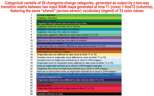
Supplemental Material
Download MS Word (51.1 KB)Data availability statement
Data sharing is not applicable to this article as no new data were created or analyzed in this study.