

Figures & data
Figure 45. National Oceanic and Atmospheric Administration (NOAA)’s Geostationary Operational Environmental Satellites (GOES)-16 Advanced Baseline Imager (ABI), 16-band spectral resolution. Temporal resolution: 5–15 minutes. Spatial resolution: Bands 1, 500 m (0.5 km), Band 2 to 5: 1000 m (1 km), Bands 6–16: 2000 m (2 km). Table legend: Visible green/red channels: G, R. Near/Middle Infrared channel: NIR, MIR. Far/Thermal Infrared: TIR, see Figure 7 in the Part 1. Top-of-atmosphere reflectance, in range [0.0, 1.0]: TOARF. Kelvin degrees, in range ≥ 0: K°.
![Figure 45. National Oceanic and Atmospheric Administration (NOAA)’s Geostationary Operational Environmental Satellites (GOES)-16 Advanced Baseline Imager (ABI), 16-band spectral resolution. Temporal resolution: 5–15 minutes. Spatial resolution: Bands 1, 500 m (0.5 km), Band 2 to 5: 1000 m (1 km), Bands 6–16: 2000 m (2 km). Table legend: Visible green/red channels: G, R. Near/Middle Infrared channel: NIR, MIR. Far/Thermal Infrared: TIR, see Figure 7 in the Part 1. Top-of-atmosphere reflectance, in range [0.0, 1.0]: TOARF. Kelvin degrees, in range ≥ 0: K°.](/cms/asset/dbb1ba66-025c-40d6-ae74-6344b117f519/tbed_a_2017582_f0001_c.jpg)
Figure 46. Active fire land cover (LC) class-specific (LC class-conditional) sample of 311 pixels selected world-wide, National Oceanic and Atmospheric Administration (NOAA)’s Geostationary Operational Environmental Satellites (GOES)-16 imaging sensor’s bands 1 to 6 (see ), radiometrically calibrated into top-of-atmosphere (TOA) reflectance (TOARF) values, belonging to the physical range of change [0.0, 1.0] (Rocha de Carvalho, Citation2019). (a) Active fire LC class-specific family (envelope) of spectral signatures, including Band 4 – Cirrus band, consisting of, first, a multivariate shape information component and, second, a multivariate intensity information component, see Figure 30 in the Part 1. To be modeled as a hyperpolyhedron, belonging to a multi-spectral (MS), specifically, a 6-dimensional, color data hypercube in TOARF values, see Figure 29 in the Part 1. (b) Same as (a), without Band 4 – Cirrus band.
![Figure 46. Active fire land cover (LC) class-specific (LC class-conditional) sample of 311 pixels selected world-wide, National Oceanic and Atmospheric Administration (NOAA)’s Geostationary Operational Environmental Satellites (GOES)-16 imaging sensor’s bands 1 to 6 (see Figure 45), radiometrically calibrated into top-of-atmosphere (TOA) reflectance (TOARF) values, belonging to the physical range of change [0.0, 1.0] (Rocha de Carvalho, Citation2019). (a) Active fire LC class-specific family (envelope) of spectral signatures, including Band 4 – Cirrus band, consisting of, first, a multivariate shape information component and, second, a multivariate intensity information component, see Figure 30 in the Part 1. To be modeled as a hyperpolyhedron, belonging to a multi-spectral (MS), specifically, a 6-dimensional, color data hypercube in TOARF values, see Figure 29 in the Part 1. (b) Same as (a), without Band 4 – Cirrus band.](/cms/asset/867c8492-64d4-4ccc-9b95-e78be3f47533/tbed_a_2017582_f0002_c.jpg)
Figure 47. Active fire land cover (LC) class-specific (LC class-conditional) sample of 311 pixels selected world-wide, National Oceanic and Atmospheric Administration (NOAA)’s Geostationary Operational Environmental Satellites (GOES)-16 imaging sensor’s bands 7 to 16 (see ), radiometrically calibrated into top-of-atmosphere (TOA) Temperature (TOAT) values, where the adopted physical unit of measure is the Kelvin degree, whose domain of variation is ≥ 0 (Rocha de Carvalho, Citation2019). This Active fire LC class-specific family (envelope) of spectral signatures consists of, first, a multivariate shape information component and, second, a multivariate intensity information component, see Figure 30 in the Part 1. To be modeled as a hyperpolyhedron, belonging to a multi-spectral (MS), specifically, a 10-dimensional, color data hypercube in Kelvin degree values, see Figure 29 in the Part 1.
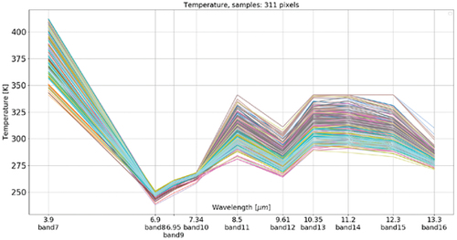
Figure 48. (a) Moderate Resolution Imaging Spectroradiometer (MODIS) image acquired on August 23, 2007, at 9.35 (CEST), covering Greece, depicted in false colors (monitor-typical channel R = MODIS band 6 in the Middle Infrared, channel G = MODIS band 2 in the Near Infrared, channel B = MODIS band 3 in the Visible Blue), spatial resolution: 1 km, radiometrically calibrated into top-of-atmosphere reflectance (TOARF) values, where an Environment for Visualizing Images (ENVI, by L3Harris Geospatial) standard histogram stretching was applied for visualization purposes. (b) Satellite Image Automatic Mapper (SIAM™)’s map of color names (Baraldi, Citation2017, Citation2019a; Baraldi et al., Citation2018a, Citation2018b, Citation2006; Baraldi & Tiede, Citation2018a, Citation2018b), generated from the MODIS image shown in (a), consisting of 83 spectral categories, depicted in pseudo-colors, refer to the SIAM map legend shown in and .
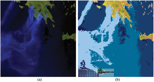
Figure 49. At left, portion of the image shown in , radiometrically calibrated into top-of-atmosphere reflectance (TOARF) values. Moderate Resolution Imaging Spectroradiometer (MODIS) image acquired on August 23, 2007, at 9.35 (CEST), covering Greece, depicted in false colors (monitor-typical channel R = MODIS band 6 in the Middle Infrared, channel G = MODIS band 2 in the Near Infrared, channel B = MODIS band 3 in the Visible Blue), spatial resolution: 1 km, radiometrically calibrated into top-of-atmosphere reflectance (TOARF) values, where an Environment for Visualizing Images (ENVI, by L3Harris Geospatial) standard histogram stretching was applied for visualization purposes. At right, Map Legend – Red: fire pixel detected in both the traditional MODIS Fire Detection (MOFID) algorithm and the SOIL MAPPER-based Fire Detection (SOMAFID) algorithm, an expert system for thermal anomalies detection (Pellegrini, Natali, & Baraldi, Citation2008). White: fire pixel detected by SOMAFID, exclusively. Green: fire pixel detected by MOFID, exclusively.
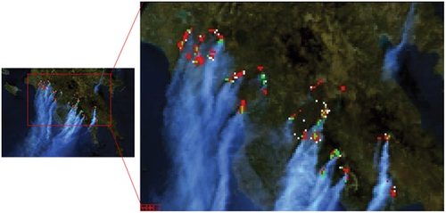
Figure 50. Legend (vocabulary) of hyperspectral color names adopted by the prior knowledge-based Landsat-like Satellite Image Automatic Mapper™ (L-SIAM™, release 88 version 7, see ) lightweight computer program for multi-spectral (MS) reflectance space hyperpolyhedralization (see Figures 29 and 30 in the Part 1), superpixel detection (see Figure 31 in the Part 1) and object-mean view (piecewise-constant input image approximation) quality assessment (Baraldi, Citation2017, Citation2019a; Baraldi et al., Citation2006, Citation2010a, Citation2010b, Citation2018a, Citation2018b; Baraldi & Tiede, Citation2018a, Citation2018b). Noteworthy, hyperspectral color names do not exist in human languages. Since humans employ a visible RGB imaging sensor as visual data source, human languages employ eleven basic color (BC) names, investigated by linguistics (Berlin & Kay, Citation1969), to partition an RGB data space into polyhedra, which are intuitive to think of and easy to visualize, see Figure 29 in the Part 1. On the contrary, hyperspectral color names (see Figure 30 in the Part 1) must be made up with (invented as) new words, not-yet existing in human languages, to be community-agreed upon for correct (conventional) interpretation before use by members of a community (refer to Subsection 4.2 in the Part 1). For the sake of representation compactness, pseudo-colors associated with the 96 color names/spectral categories, corresponding to a partition of the MS reflectance hyperspace into a discrete and finite ensemble of mutually exclusive and totally exhaustive hyperpolyhedra, equivalent to 96 envelopes/families of spectral signatures (see Figures 29 and 30 in the Part 1), are gathered along the same raw if they share the same parent spectral category (parent hyperpolyhedron) in the prior knowledge-based (static, non-adaptive to data) SIAM decision tree, e.g. “strong” vegetation, equivalent to a spectral end-member (Adams et al., Citation1995). The pseudo-color of a spectral category (color name) is chosen to mimic natural RGB colors of pixels belonging to that spectral category (Baraldi, Citation2017, Citation2019a; Baraldi et al., Citation2006, Citation2010a, Citation2010b, Citation2018a, Citation2018b; Baraldi & Tiede, Citation2018a, Citation2018b).
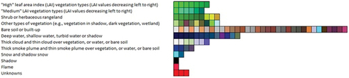
Figure 51. (a) False color quick-look Red-Green-Blue (RGB) Sentinel-2A Multi-Spectral Instrument (MSI) image Level-1C, calibrated into top-of-atmosphere reflectance (TOARF) values, depicting a surface area in SE Australia, acquired on 2019-12-31. In particular: R = Middle Infrared (MIR) = Band 11, G = Near Infrared (NIR) = Band 8, B = Visible Blue = Band 2. Spatial resolution: 10 m. No histogram stretching is applied for visualization purposes. (b) Same as Figure (a), followed by an Environment for Visualizing Images (ENVI, by L3Harris Geospatial) standard histogram stretching, applied for visualization purposes. (c) SIAM’s map of color names generated from Figure (a), consisting of 96 spectral categories (color names) depicted in pseudo-colors. Map of color names legend: 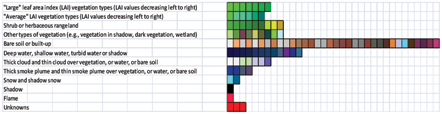
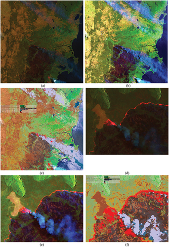
Figure 52. Multi-spectral (MS) signature in top-of-atmosphere reflectance (TOARF) values in range [0, 1], byte-coded into range {0, 255}, such that TOARF_byte = BYTE(TOARF_float * 255.0 + 0.5), where TOARF_byte ∈ {0, 255} is affected by a discretization (quantization) error = (TOARF_Max – TOARF_Min)/255 bins/2 (due to rounding to the closest integer, either above or below) = (1.0–0.0)/255.0/2.0 = 0.002 = 0.2%, to be considered negligible (Baraldi, Citation2017, Citation2019a; Baraldi et al., Citation2006, Citation2010a, Citation2010b, Citation2018a, Citation2018b; Baraldi & Tiede, Citation2018a, Citation2018b) (refer to Subsection 3.3.2 in the Part 1). (a) Active fire samples (region of interest, ROI), MS signature in TOARF_byte values in range {0, 255}, Sentinel-2A Multi-Spectral Instrument (MSI) image Level-1C, of Australia, acquired on 2019-12-31 and shown in , with bands 1 to 6 equivalent to Landsat-7 ETM+ bands 1 to 5 and 7, respectively. No thermal channel is available in Sentinel-2 MSI imagery, equivalent to the Landsat 7 ETM+ channels 61 and/or 62. (b) For comparison purposes with Figure (a), active fire samples, whose MS signature in TOARF_byte values belongs to range {0, 255}, are selected from a Landsat 7 ETM+ image of Senegal, Path: 203, Row: 051, acquisition date: 2001-01-11. Thermal band ETM62 in kelvin degrees in interval [−100, 155], linearly shifted into range {0, 255}. The two sensor-specific active fire spectral signatures in TOARF values shown in Figure (a) and Figure (b) should be compared with those collected by the geostationary GOES-16 ABI imaging sensor, shown in and .
![Figure 52. Multi-spectral (MS) signature in top-of-atmosphere reflectance (TOARF) values in range [0, 1], byte-coded into range {0, 255}, such that TOARF_byte = BYTE(TOARF_float * 255.0 + 0.5), where TOARF_byte ∈ {0, 255} is affected by a discretization (quantization) error = (TOARF_Max – TOARF_Min)/255 bins/2 (due to rounding to the closest integer, either above or below) = (1.0–0.0)/255.0/2.0 = 0.002 = 0.2%, to be considered negligible (Baraldi, Citation2017, Citation2019a; Baraldi et al., Citation2006, Citation2010a, Citation2010b, Citation2018a, Citation2018b; Baraldi & Tiede, Citation2018a, Citation2018b) (refer to Subsection 3.3.2 in the Part 1). (a) Active fire samples (region of interest, ROI), MS signature in TOARF_byte values in range {0, 255}, Sentinel-2A Multi-Spectral Instrument (MSI) image Level-1C, of Australia, acquired on 2019-12-31 and shown in Figure 51, with bands 1 to 6 equivalent to Landsat-7 ETM+ bands 1 to 5 and 7, respectively. No thermal channel is available in Sentinel-2 MSI imagery, equivalent to the Landsat 7 ETM+ channels 61 and/or 62. (b) For comparison purposes with Figure (a), active fire samples, whose MS signature in TOARF_byte values belongs to range {0, 255}, are selected from a Landsat 7 ETM+ image of Senegal, Path: 203, Row: 051, acquisition date: 2001-01-11. Thermal band ETM62 in kelvin degrees in interval [−100, 155], linearly shifted into range {0, 255}. The two sensor-specific active fire spectral signatures in TOARF values shown in Figure (a) and Figure (b) should be compared with those collected by the geostationary GOES-16 ABI imaging sensor, shown in Figures 46 and 47.](/cms/asset/51c644e8-a12a-42f6-9464-58ecd2c91320/tbed_a_2017582_f0008_c.jpg)
Figure 53. Ideal Earth observation (EO) optical sensory data-derived Level 2/Analysis Ready Data (ARD) product generation system design as a hierarchical alternating sequence of: (A) hybrid (combined deductive and inductive) class-conditional radiometric enhancement of EO Level 1 multi-spectral (MS) top-of-atmosphere reflectance (TOARF) values into EO Level 2/ARD surface reflectance (SURF) 1-of-3, SURF 2-of-3, SURF 3-of-3 and surface albedo values (EC – European Commission, Citation2020; Li et al., Citation2012; Malenovsky et al., Citation2007; Schaepman-Strub et al., Citation2006; Shuai et al., Citation2020) corrected in sequence for (1) atmospheric, (5) topographic (6) adjacency and (7) bidirectional reflectance distribution function (BRDF) effects (Egorov, Roy, Zhang, Hansen, & Kommareddy, Citation2018), and (B) hybrid (combined deductive and inductive) classification of TOARF, SURF 1-of-3 to SURF 3-of-3 and surface albedo values into a stepwise sequence of EO Level 2/ARD scene classification maps (SCMs), whose legend (taxonomy) of community-agreed land cover (LC) class names, in addition to quality layers Cloud and Cloud–shadow, increases stepwise in mapping accuracy and/or in semantics, i.e. stepwise, it reaches deeper semantic levels/finer semantic granularities in a hierarchical LC class taxonomy, see Figure 3 in the Part 1. An instantiation of this EO image pre-processing system design for EO Level 2/ARD symbolic and subsymbolic co-products generation is depicted in . In comparison with this desirable system design, the existing ESA Sen2Cor software system design (see Figure 38 in the Part 1) adopts no hierarchical alternating approach between MS image classification and MS image radiometric enhancement. In more detail, it accomplishes, first, one SCM generation from TOARF values based on a per-pixel (2D spatial context-insensitive) prior spectral knowledge-based decision-tree classifier (synonym for static/non-adaptive-to-data decision-tree for MS color naming, see Figures 29 and 30 in the Part 1). Next, in the ESA Sen2Cor workflow, a stratified/class-conditional MS image radiometric enhancement of TOARF into SURF 1-of-3 up to SURF 3-of-3 values corrected for atmospheric, topographic and adjacency effects is accomplished in sequence, stratified (class-conditioned) by (the haze map and cirrus map of) the same SCM product generated at first stage from TOARF values. In summary, the ESA Sen2Cor SCM co-product is TOARF-derived; hence, it is not “aligned” with data in the ESA Sen2Cor output MS image co-product, consisting of TOARF values radiometrically corrected into SURF 3-of-3 values (refer to Subsection 3.3.2 in the Part 1), where, typically, SURF ≠ TOARF holds, see Equation (9) in the Part 1.
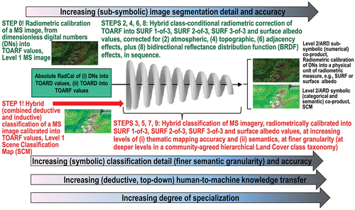
Figure 54. The well-known engineering principles of modularity, hierarchy and regularity, recommended for system scalability (Lipson, Citation2007), characterize a single-date EO optical image processing system design for state-of-the-art multi-sensor EO data-derived Level 2/Analysis Ready Data (ARD) product generation, encompassing an ARD-specific symbolic co-product, known as Scene Classification Map (SCM) (refer to Subsection 8.1.1), and an ARD-specific numerical co-product (refer to Subsection 8.1.2) to be estimated alternately and hierarchically, see . Stage 1: Absolute radiometric calibration (Cal) of dimensionless Digital Numbers (DNs) into top-of-atmosphere (TOA) radiance (TOARD) values ≥ 0. Stage 2: Cal of TOARD into TOA reflectance (TOARF) values ∈ [0.0, 1.0]. Stage 3: EO image classification by an automatic computer vision (CV) system, based on a convergence of spatial with colorimetric evidence (refer to Subsection 4.1 in the Part 1). Stage 4: Class-conditional/Stratified atmospheric correction of TOARF into surface reflectance (SURF) 1-of-3 values ∈ [0, 1]. Stage 5: Class-conditional/Stratified Topographic Correction (STRATCOR) of SURF 1-of-3 into SURF 2-of-3 values. Stage 6: Class-conditional/Stratified adjacency effect correction of SURF 2-of-3 into SURF 3-of-3 values. Stage 7: Class-conditional/Stratified bidirectional reflectance distribution function (BRDF) effect correction of SURF 3-of-3 values into surface albedo values (Bilal et al., Citation2019; EC – European Commission, Citation2020; Egorov, Roy, Zhang, Hansen, & Kommareddy, Citation2018; Franch et al., Citation2019; Li et al., Citation2012; Malenovsky et al., Citation2007; Qiu et al., Citation2019; Schaepman-Strub et al., Citation2006; Shuai et al., Citation2020). This original ARD system design is alternative to, for example, the EO image processing system design and implementation proposed in (Qiu et al., Citation2019) where, to augment the temporal consistency of USGS Landsat ARD imagery, neither topographic correction nor BRDF effect correction is land cover (LC) class-conditional. Worth mentioning, both SCM (referred to as land cover) and surface albedo (referred to as albedo) are included in the list of terrestrial Essential Climate Variables (ECVs) defined by the World Climate Organization (WCO) (Bojinski et al., Citation2014) (see Table 2 in the Part 1), which complies with the Group on Earth Observations (GEO)’s second implementation plan for years 2016–2025 of a new Global Earth Observation System of (component) Systems (GEOSS) as expert EO data-derived information and knowledge system (GEO – Group on Earth Observations, Citation2015; Nativi et al., Citation2015, Citation2020; Santoro et al., Citation2017), see Figure 1 in the Part 1.
![Figure 54. The well-known engineering principles of modularity, hierarchy and regularity, recommended for system scalability (Lipson, Citation2007), characterize a single-date EO optical image processing system design for state-of-the-art multi-sensor EO data-derived Level 2/Analysis Ready Data (ARD) product generation, encompassing an ARD-specific symbolic co-product, known as Scene Classification Map (SCM) (refer to Subsection 8.1.1), and an ARD-specific numerical co-product (refer to Subsection 8.1.2) to be estimated alternately and hierarchically, see Figure 53. Stage 1: Absolute radiometric calibration (Cal) of dimensionless Digital Numbers (DNs) into top-of-atmosphere (TOA) radiance (TOARD) values ≥ 0. Stage 2: Cal of TOARD into TOA reflectance (TOARF) values ∈ [0.0, 1.0]. Stage 3: EO image classification by an automatic computer vision (CV) system, based on a convergence of spatial with colorimetric evidence (refer to Subsection 4.1 in the Part 1). Stage 4: Class-conditional/Stratified atmospheric correction of TOARF into surface reflectance (SURF) 1-of-3 values ∈ [0, 1]. Stage 5: Class-conditional/Stratified Topographic Correction (STRATCOR) of SURF 1-of-3 into SURF 2-of-3 values. Stage 6: Class-conditional/Stratified adjacency effect correction of SURF 2-of-3 into SURF 3-of-3 values. Stage 7: Class-conditional/Stratified bidirectional reflectance distribution function (BRDF) effect correction of SURF 3-of-3 values into surface albedo values (Bilal et al., Citation2019; EC – European Commission, Citation2020; Egorov, Roy, Zhang, Hansen, & Kommareddy, Citation2018; Franch et al., Citation2019; Li et al., Citation2012; Malenovsky et al., Citation2007; Qiu et al., Citation2019; Schaepman-Strub et al., Citation2006; Shuai et al., Citation2020). This original ARD system design is alternative to, for example, the EO image processing system design and implementation proposed in (Qiu et al., Citation2019) where, to augment the temporal consistency of USGS Landsat ARD imagery, neither topographic correction nor BRDF effect correction is land cover (LC) class-conditional. Worth mentioning, both SCM (referred to as land cover) and surface albedo (referred to as albedo) are included in the list of terrestrial Essential Climate Variables (ECVs) defined by the World Climate Organization (WCO) (Bojinski et al., Citation2014) (see Table 2 in the Part 1), which complies with the Group on Earth Observations (GEO)’s second implementation plan for years 2016–2025 of a new Global Earth Observation System of (component) Systems (GEOSS) as expert EO data-derived information and knowledge system (GEO – Group on Earth Observations, Citation2015; Nativi et al., Citation2015, Citation2020; Santoro et al., Citation2017), see Figure 1 in the Part 1.](/cms/asset/e0975773-9d6d-4c18-a2da-1a711c614766/tbed_a_2017582_f0010_c.jpg)
Figure 55. Top left: Red-Green-Blue (RGB) image, source: Akiyoshi Kitaoka @AkiyoshiKitaoka, web page: http://nymag.com/selectall/2017/02/strawberries-look-red-without-red-pixels-color-constancy.html. Strawberries appear to be reddish, though the pixels are not, refer to the monitor-typical RGB input-output histograms shown at bottom left. No histogram stretching is applied for visualization purposes, see the monitor-typical RGB input-output histograms shown at bottom left. Top right: Output of the self-organizing statistical model-based color constancy algorithm, as reported in (Baraldi, Citation2017; Baraldi & Tiede, Citation2018a, Citation2018b; Baraldi et al., Citation2017; Vo et al., Citation2016), input with the image shown top left. No histogram stretching is applied for visualization purposes, see the monitor-typical RGB input-output histograms shown at bottom right.
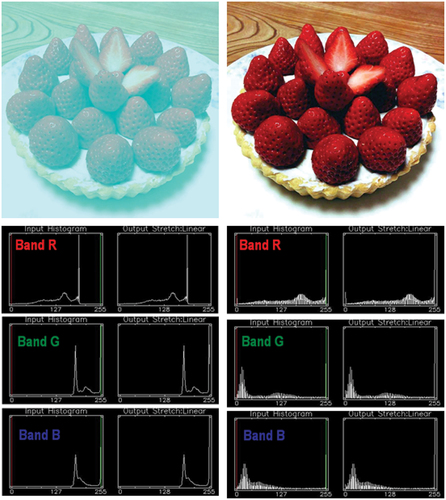
Figure 56. Fully automated two-stage stratified (class-conditional) topographic correction (STRATCOR) (Baraldi et al., Citation2010). (a) Zoomed area of a Landsat 7 ETM+ image of Colorado, USA (path: 128, row: 021, acquisition date: 2000–08-09), depicted in false colors (R: band ETM5, G: band ETM4, B: band ETM1), 30 m resolution, radiometrically calibrated into TOARF values. (b) STRATCOR applied to the Landsat image shown at left, with data stratification based on the Shuttle Radar Topography Mission (SRTM) Digital Elevation Model (DEM) and a 18-class preliminary spectral map generated at coarse granularity by the 7-band Landsat-like Satellite Image Automatic Mapper (L-SIAM) software toolbox (Baraldi, Citation2017, Citation2019a; Baraldi et al., Citation2006, Citation2010a, Citation2010b, Citation2018a, Citation2018b; Baraldi & Tiede, Citation2018a, Citation2018b), see .
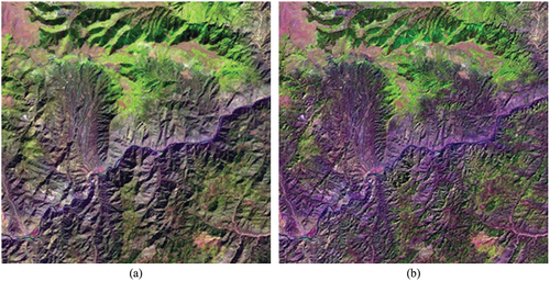
Figure 57. (a) Meteosat Second Generation (MSG) Spinning Enhanced Visible and InfraRed Imager (SEVIRI) image acquired on 2012-05-30, radiometrically calibrated into TOARF values and depicted in false colors (R: band MIR, G: band NIR, B: band Blue), spatial resolution: 3 km. No histogram stretching is applied for visualization purposes. (b). Advanced Very High Resolution Radiometer (AVHRR)-like SIAM (AV-SIAM™, release 88 version 7) hyperpolyhedralization of the MS reflectance hyperspace and prior knowledge-based mapping of the input MS image into a vocabulary of hypercolor names. The AV-SIAM map legend, consisting of 83 spectral categories (see ), is depicted in pseudo-colors, similar to those shown in : 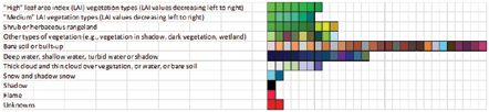
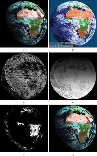
Figure 58. (a) Airborne 10 cm resolution true-color Red-Green-Blue (RGB) orthophoto of Trento, Italy, 4017 × 4096 pixels in size x 3 bands, acquired in 2014 and provided with no radiometric calibration metadata file. No histogram stretching is applied for visualization purposes. (b) Same RGB orthophoto, subject to self-organizing statistical color constancy (Baraldi, Citation2017; Baraldi & Tiede, Citation2018a, Citation2018b; Baraldi et al., Citation2017; Vo et al., Citation2016). No histogram stretching is applied for visualization purposes. (c) RGBIAM’s polyhedralization of the RGB color space and prior knowledge-based map of RGB color names generated from the RGB image, pre-processed by a color constancy algorithm (Baraldi, Citation2017; Baraldi & Tiede, Citation2018a, Citation2018b; Baraldi et al., Citation2017; Vo et al., Citation2016). The RGBIAM legend of RGB color names, consisting of 50 spectral categories at fine discretization granularity, is depicted in pseudo-colors. Map legend, shown in : 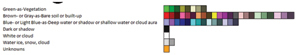
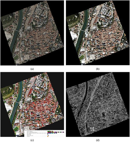
Figure 59. Legend (vocabulary) of RGB color names adopted by the prior knowledge-based Red-Green-Blue (RGB) Image Automatic Mapper™ (RGBIAM™, release 6 version 2) lightweight computer program for RGB data space polyhedralization (see Figure 29 in the Part 1), superpixel detection (see Figure 31 in the Part 1) and object-mean view (piecewise-constant input image approximation) quality assessment (Baraldi, Citation2017, Citation2019a; Baraldi et al., Citation2006; Citation2018a, Citation2018b; Baraldi & Tiede, Citation2018a, Citation2018b). Before running RGBIAM to map onto a deterministic RGB color name each pixel value of an input 3-band RGB image, encoded in either true- or false-colors, the RGB image should be pre-processed (enhanced) for normalization/ harmonization/ calibration (Cal) purposes, e.g. by means of a color constancy algorithm (Baraldi, Citation2017; Baraldi & Tiede, Citation2018a, Citation2018b; Baraldi et al., Citation2017; Boynton, Citation1990; Finlayson et al., Citation2001; Gevers et al., Citation2012; Gijsenij et al., Citation2010; Vo et al., Citation2016), see and . The RGBIAM implementation (release 6 version 2) adopts 12 basic color (BC) names (polyhedra) as coarse RGB color space partitioning, consisting of the eleven BC names adopted by human languages (Berlin & Kay, Citation1969), specifically, black, white, gray, red, orange, yellow, green, blue, purple, pink and brown (refer to Subsection 4.2 in the Part 1), plus category “Unknowns” (refer to Section 2 in the Part 1), and 50 color names as fine color quantization (discretization) granularity, featuring parent-child relationships from the coarse to the fine quantization level. For the sake of representation compactness, pseudo-colors associated with the 50 color names (spectral categories, corresponding to a mutually exclusive and totally exhaustive partition of the RGB data space into polyhedra, see Figure 29 in the Part 1) are gathered along the same raw if they share the same parent spectral category (parent polyhedron) in the prior knowledge-based (static, non-adaptive to data) RGBIAM decision tree. The pseudo-color of a spectral category (color name) is chosen to mimic natural RGB colors of pixels belonging to that spectral category (Baraldi, Citation2017; Baraldi & Tiede, Citation2018a, Citation2018b; Baraldi et al., Citation2017; Vo et al., Citation2016).
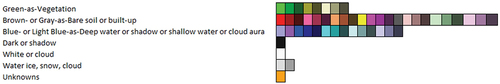
Figure 60. First test image of a Cambodia site (Baraldi & Tiede, Citation2018b). Final 3-level Cloud/Cloud–shadow/Others maps generated by the three algorithms under comparison, specifically, single-date AutoCloud+, the single-date AutoCloud+ Baraldi & Tiede, Citation2018a, Citation2018b), the single-date Sen2Cor (DLR - Deutsches Zentrum für Luft-und Raumfahrt e.V. and VEGA Technologies, Citation2011; ESA - European Space Agency, Citation2015) and the multi-date MAJA (Hagolle et al., Citation2017; Main-Knorn et al., Citation2018), where class “Others” is overlaid with the input Sentinel-2 A Multi-Spectral Instrument (MSI) Level 1C image, radiometrically calibrated into top-of-atmosphere reflectance (TOARF) values and depicted in false-colors: monitor-typical Red-Green-Blue (RGB) channels are selected as R = Near Infrared (NIR) channel, G = Visible Red channel, B = Visible Green channel. Histogram stretching is applied for visualization purposes. Output class Cloud is shown in a green pseudo-color, class Cloud–shadow in a yellow pseudo-color.
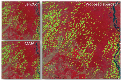
Figure 61. First test image of a Cambodia site (Baraldi & Tiede, Citation2018b). Zoom-in of the final 3-level Cloud/Cloud–shadow/Others maps generated by the three algorithms under comparison, where class “others” is overlaid with the input Sentinel-2 A Multi-Spectral Instrument (MSI) Level 1C image, radiometrically calibrated into top-of-atmosphere (TOA) reflectance (TOARF) values and depicted in false-colors: monitor-typical RGB channels are selected as R = Near InfraRed (NIR) channel, G = Visible Red channel, B = Visible Green channel. Histogram stretching is applied for visualization purposes. Output class Cloud is shown in a green pseudo-color, class Cloud–shadow in a yellow pseudo-color. Based on qualitative photointerpetation, the single-date Sen2Cor algorithm (DLR - Deutsches Zentrum für Luft-und Raumfahrt e.V. and VEGA Technologies, Citation2011; ESA - European Space Agency, Citation2015) appears to underestimate Cloud–shadows, although some Water areas are misclassified as Cloud–shadow. In addition, some River/river beds are misclassified as Cloud. These two cases of Cloud false positives and Cloud–shadow false positives are highlighted in blue circles. The multi-date MAJA algorithm (Hagolle et al., Citation2017; Main-Knorn et al., Citation2018), overlooks some Cloud instances small in size (in relative terms), as highlighted in red circles.
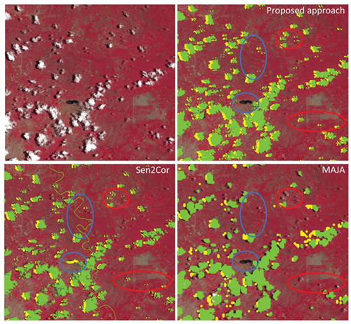
Figure 62. First test image of a Cambodia site (Baraldi & Tiede, Citation2018b). Extra zoom-in of the final 3-level Cloud/Cloud–shadow/Others maps generated by the three algorithms under comparison, where class “Others” is overlaid with the input Sentinel-2 A Multi-Spectral Instrument (MSI) Level 1C image, radiometrically calibrated into top-of-atmosphere (TOA) reflectance (TOARF) values and depicted in false-colors: monitor-typical RGB channels are selected as R = Near InfraRed (NIR) channel, G = Visible Red channel, B = Visible Green channel. Histogram stretching is applied for visualization purposes. Output class Cloud is shown in a green pseudo-color, class Cloud–shadow in a yellow pseudo-color. Based on qualitative photointerpetation, the single-date Sen2Cor algorithm (DLR - Deutsches Zentrum für Luft-und Raumfahrt e.V. and VEGA Technologies, Citation2011; ESA - European Space Agency, Citation2015) appears to underestimate class Cloud–shadow, although some detected Cloud–shadow instances are false positives because of misclassified Water areas. In addition, some River/river beds are misclassified as Cloud. To reduce false positives in Cloud–shadow detection, MAJA adopts a multi-date approach. Nevertheless, the multi-date MAJA algorithm (Hagolle et al., Citation2017; Main-Knorn et al., Citation2018), misses some instances of Cloud-over-water. Overall, MAJA’s Cloud and Cloud–shadow results look more “blocky” (affected by artifacts in localizing true boundaries of target image-objects).
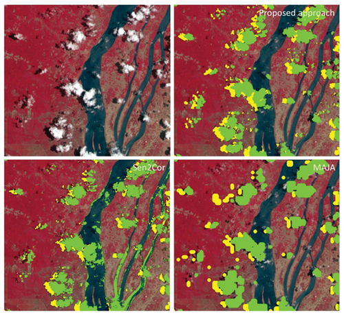
Figure 63. Typical values of a minimally dependent maximally informative (mDMI) set of outcome and process quantitative quality indicators (OP-Q2Is) featured by a pixel-based (2D spatial context-insensitive) 1D image analysis algorithm (see Figure 18 in the Part 1) for Cloud and Cloud-shadow detection in MS imagery (see Figure 22 in the Part 1), such as Fmask (Zhu et al., Citation2015), ESA Sen2Cor (DLR – Deutsches Zentrum für Luft-und Raumfahrt e.V. and VEGA Technologies, Citation2011; ESA – European Space Agency, Citation2015) and CNES-DLR MAJA (Hagolle et al., Citation2017; Main-Knorn et al., Citation2018) (see ), considered a mandatory EO image understanding (classification) task for quality layers detection in Analysis Ready Data (ARD) workflows.
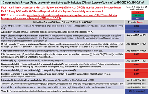
Figure 64. Typical values of a minimally dependent maximally informative (mDMI) set of outcome and process quantitative quality indicators (OP-Q2Is) featured by a deep convolutional neural network (DCNN) (Cimpoi et al., Citation2014) involved with Cloud and Cloud-shadow detection in MS imagery (Bartoš, Citation2017; EOportal, Citation2020; Wieland et al., Citation2019) (see ), considered a mandatory EO image understanding (classification) task for quality layers detection in Analysis Ready Data (ARD) workflows.
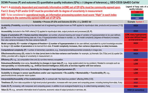
Figure 65. Expected values of a minimally dependent maximally informative (mDMI) set of outcome and process quantitative quality indicators (OP-Q2Is) featured by a “universal” multi-sensor automatic AutoCloud+ algorithm for Cloud and Cloud-shadow detection in multi-spectral (MS) imagery (Baraldi & Tiede, Citation2018a, Citation2018b) (see ), considered a mandatory EO image understanding (classification) task for quality layers detection in Analysis Ready Data (ARD) workflows. By scoring “high” in each indicator of an mDMI set of OP-Q2Is, a “universal” multi-sensor automated AutoCloud+ algorithm for Cloud and Cloud-shadow quality layers detection in MS imagery is expected to be considered in operational mode (Baraldi, Citation2017; Baraldi & Tiede, Citation2018a, Citation2018b), as necessary-but-not-sufficient precondition of ARD workflows.
Table 4. The Satellite Image Automatic Mapper™ (SIAM™) lightweight computer program (release 88 version 7) for multi-spectral (MS) reflectance space hyperpolyhedralization (see Figures 29 and 30 in the Part 1), superpixel detection (see Figure 31 in the Part 1) and object-mean view quality assessment (Baraldi, Citation2017, Citation2019a; Baraldi et al., Citation2006, Citation2010a, Citation2010b, Citation2018a, Citation2018b; Baraldi & Tiede, Citation2018a, Citation2018b). SIAM is an Earth observation (EO) system of systems scalable to any past, present or future MS imaging sensor, provided with radiometric calibration metadata parameters for radiometric calibration (Cal) of digital numbers into top-of-atmosphere reflectance (TOARF), surface reflectance (SURF) or surface albedo values, where relationship ‘TOARF ⊇ SURF ⊇ Surface albedo’ = Equation (8) in the Part 1 holds. SIAM is an expert system (deductive/ top-down/ prior knowledge-based static decision tree, non-adaptive to input data) for mapping each color value in the MS reflectance space into a color name belonging to the SIAM vocabulary of hypercolor names. It consists of the following subsystems. (i) 7-band Landsat-like SIAM™ (L-SIAM™), with Landsat-like input channels Blue (B) = Blue0.45÷0.50, Green (G) = Green0.54÷0.58, Red (R) = Red0.65÷0.68, Near Infrared (NIR) = NIR0.78÷0.90, Middle Infrared 1 (MIR1) = MIR1.57÷1.65, Middle Infrared 2 (MIR2) = MIR2.08÷2.35, and Thermal Infrared (TIR) = TIR10.4–12.5, see Figure 7 and Table 3 in the Part 1. (ii) 4-band (channels G, R, NIR, MIR1) SPOT-like SIAM™ (S-SIAM™). (iii) 4-band (channels R, NIR, MIR1, and TIR) Advanced Very High Resolution Radiometer (AVHRR)-like SIAM™ (AV-SIAM™). (iv) 4-band (channels B, G, R, and NIR) QuickBird-like SIAM™ (Q-SIAM™) (Baraldi, Citation2017, Citation2019a; Baraldi et al., Citation2006, Citation2010a, Citation2010b, Citation2018a, Citation2018b; Baraldi & Tiede, Citation2018a, Citation2018b).
Table 5. Conceptual/methodological comparison of existing algorithms for Cloud and Cloud-shadow quality layers detection in spaceborne MS imagery for EO Level 2/ARD-specific symbolic output co-product generation.
Supplemental Material
Download MS Word (16.5 KB)Data availability statement
Data sharing is not applicable to this article as no new data were created or analyzed in this study.