Fine-resolution mapping of the circumpolar Arctic Man-made impervious areas (CAMI) using sentinels, OpenStreetMap and ArcticDEM

Figures & data

Figure 1. Spatial extent of the study area.

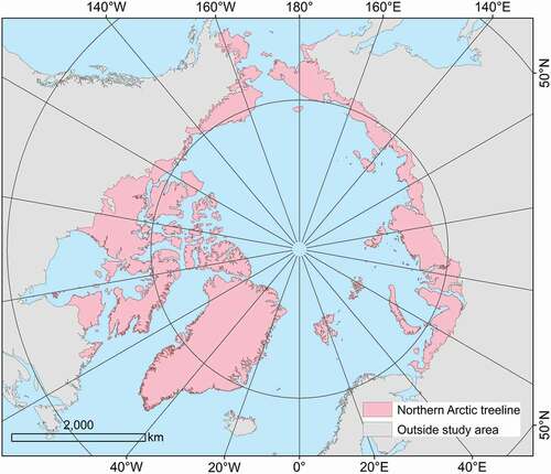
Figure 2. Workflow of our proposed approach for the CAMI mapping.

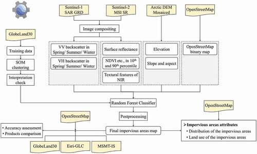
Table 1. All of 33 features used in the RF model.

Data	Features	Variable Names
Sentinel-1 SAR	Mean of VV in spring, summer and winter	VV_Spring, VV_Summer, VV_Winter
	Mean of VH in spring, summer and winter	VH_Spring, VH_Summer, VH_Winter
Sentinel-2 MSI	Reflectance: blue, green, red, red edge1,2,3,4, NIR and SWIR1,2	B2, B3, B4, B5, B6, B7, B8, B8A, B11, B12
	Normalized indices: 10^th percentile of NDVI, MNDWI and NDBI	NDVI10, MNDWI10, NDBI10
	Normalized indices: 90^th percentile of NDVI, MNDWI and NDBI	NDVI90, MNDWI90, NDBI90
	Normalized indices: mean MNDWI $-$ mean NDBI	WI_BI_diff
	Textural variables: contrast, variance, sum variance, dissimilarity, inertia and cluster prominence of the NIR	B8_Contrast, B8_Variance, B8_Sum_Variance, B8_Dissimilarity, B8_Inertia, B8_Cluster_Prominence
DEM	Elevation, slope and aspect	Elevation, Slope, Aspect
Auxiliary data	OpenStreetMap	OSM

Figure 3. Validation sampling strategy.

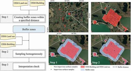
Figure 4. Distribution of impervious areas in the northern Arctic treeline. Every point in the map refers to the location of the centroid of the impervious areas and its color refers to the area. The highlighted sites in the map are located in Alaska, Canada, Russia and Greenland.

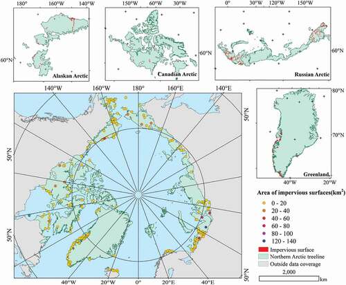
Figure 5. Distribution of zonal impervious areas calculated by $0.05°$ interval.

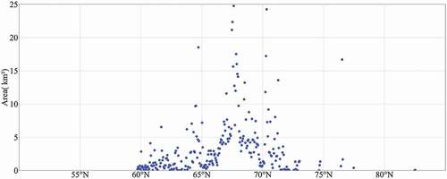
Figure 6. Distribution of meridional impervious areas calculated by $k{m}^2$ interval.

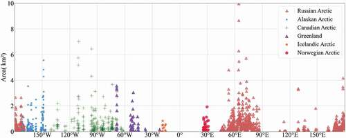
Figure 7. Impervious surfaces area in different regions.

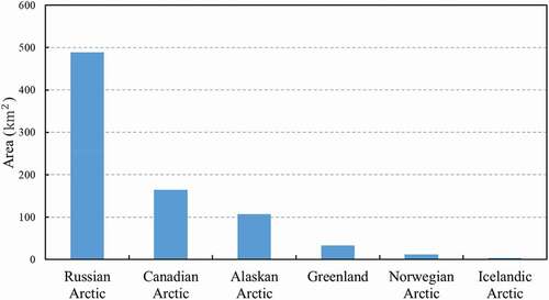
Table 2. Accuracy of the four impervious areas maps using validation samples.

		Alaskan Arctic	Canadian Arctic	Greenland	Icelandic Arctic	Norwegian Arctic	Russian Arctic	Overall
This study	O.A.	85.71%	92.59%	88.19%	85.32%	78.14%	85.09%	86.36%
	Kappa	69.94%	82.64%	73.98%	69.57%	49.43%	69.29%	70.73%
	P.I.	70.65%	82.11%	82.14%	74.74%	52.42%	74.34%	73.91%
	U.I.	94.89%	94.71%	83.94%%	89.87%	82.28%	90.52%	90.32%
	P.N.	97.12%	97.74%	91.47%	93.50%	93.33%	93.74%	94.70%
	U.N.	81.38%	91.74%	90.42%	82.73%	76.86%	81.97%	84.42%
GlobeLand30	O.A.	88.52%	90.77%	74.62%	74.31%	76.65%	84.86%	83.76%
	Kappa	76.56%	77.81%	33.88%	45.81%	44.88%	68.95%	64.82%
	P.I.	85.87%	74.31%	29.29%	54.74%	45.97%	76.46%	68.02%
	U.I.	87.29%	97.01%	95.35%	80.00%	83.82%	87.98%	88.87%
	P.N.	90.53%	98.87%	99.22%	89.43%	94.76%	91.61%	94.29%
	U.N.	89.43%	88.66%	72.11%	71.90%	74.81%	82.88%	81.49%
Esri-GLC	O.A.	73.07%	78.21%	77.39%	78.90%	70.94%	77.84%	77.50%
	Kappa	41.01%	41.82%	44.01%	54.70%	43.53%	53.41%	49.20%
	P.I.	40.76%	37.16%	42.86%	52.63%	46.77%	56.11%	48.34%
	U.I.	92.59%	92.05%	85.71%	98.04%	96.67%	90.57%	91.57%
	P.N.	97.53%	98.42%	96.12%	99.19%	98.18%	95.31%	97.02%
	U.N.	68.50%	76.09%	75.61%	73.05%	62.07%	72.98%	73.71%
MSMT-IS30	O.A.	81.03%	80.94%	/	/	73.95%	73.74%	76.69%
	Kappa	59.37%	50.28%	/	/	37.73%	44.90%	52.89%
	P.I.	58.15%	44.95%	/	/	39.52%	90.75%	72.58%
	U.I.	96.40%	94.23%	/	/	80.33%	70.42%	75.47%
	P.N.	98.35%	98.65%	/	/	94.29%	52.57%	80.15%
	U.N.	75.63%	78.46%	/	/	72.53%	82.04%	77.65%

P.I., producer’s accuracy of impervious areas, U.I., user’s accuracy of impervious areas, P.N., producer’s accuracy of non-impervious areas, U.N., user’s accuracy of non-impervious areas. MSMT-IS30 lacked of impervious areas result in Greenland and Iceland.

Figure 8. Comparison between the method result (the third column) and the three other impervious products (the 4th to 6th columns corresponded to the GlobeLand30, Esri-GLC and MSMT_IS) for six plots. The second column is the corresponding RGB-composite Sentinel-2 images in 2020.

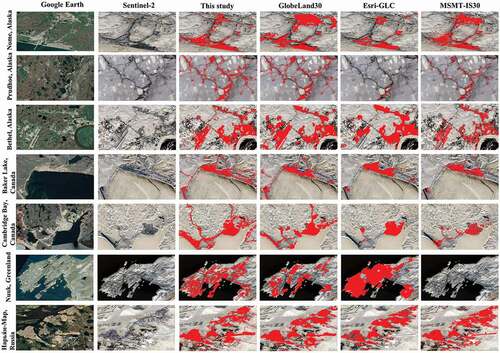
Figure 9. Area proportion of impervious land-use in Russia, Norway, Iceland, Greenland, Canada and Alaska. The impervious areas for industrial use contains industrial and mining land, for public use contains parks, cemetery and parking lots, for transport use contains airport and apron. Unclassified class refers to the impervious areas with unknown land-use identification in OSM dataset.

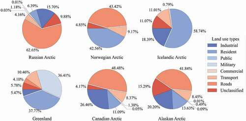
Figure 10. Stacked bar of 8 impervious land-use class in Arctic and its fraction of every country (region).

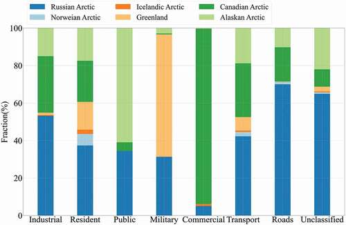
Figure 11. The importance of the input features derived from the random forest model using the training samples in six regions. Mean decrease in accuracy was used to assess the importance of the input features, which refers how much the model accuracy decreases if that variable was dropped. The bar with different colors refers the mean importance of the different data sources.

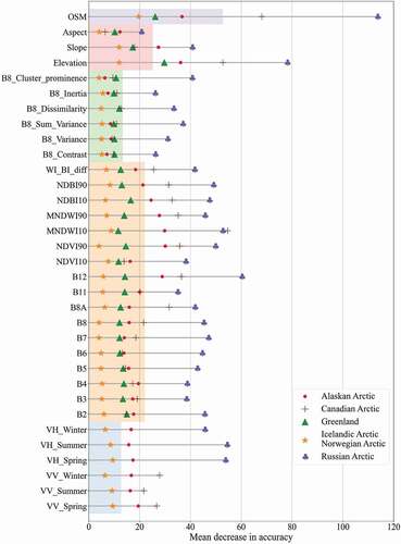
Figure 12. Example of classification results of human-impacted areas in comparison to OpenStreetMap and the Google Earth online hybrid map in Yamal, Russia: (a) OpenStreetMap (blue-waterbodies, grey-roads); (b) classification results based on this study; (c) Google Earth online hybrid map; (d) Sentinel-2 red-green-blue (band 4-3-2) composition in 2020. Projection WGS_1984_EPSG_Russia_Polar_Stereographic.

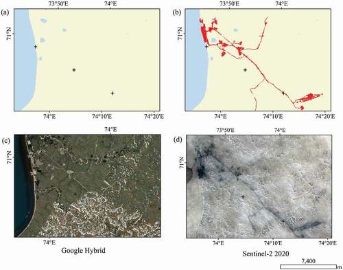
Figure 13. Examples of human-impacted areas in comparison to SAR images, Google Earth and classification result with SAR derived features only in Arctic: the first column refers the Sentinel-1 spring-summer-winter composition in 2020, the second column refers Google Earth online hybrid map and the third column refers the classification result based on the SAR derived features. The highlighted boxes in yellow indicate the true impervious areas and cyan boxes indicate the bare lands.

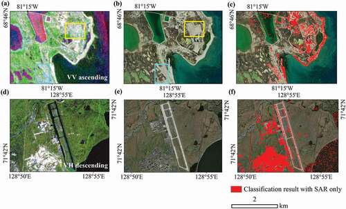
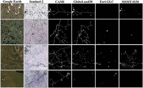
Figure 14. Roads comparison between CAMI and the three impervious surfaces products (the 4^th to 6^th columns corresponded to the GlobeLand30, Esri-GLC and MSMT_IS30) for four plots. The second column is the corresponding RGB-composite Sentinel-2 images in 2020.

Data availability statement

The CAMI map will be openly accessed at http://www.doi.org/10.11922/sciencedb.01435