
Figures & data
Figure 1. Tree-ring chronologies and their length distribution. The topography is derived from NOAA’s global 1 km DEM dataset (https://www.ngdc.noaa.gov/mgg/topo/globe.html) with the WGS 1984 geographic coordinate system and Mercator projected coordinate system. The triangular symbol represents the location of tree-ring chronologies, and the color from light to dark indicates the length from short to long, respectively.
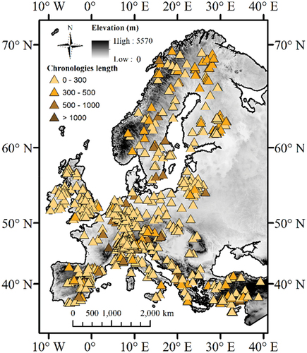
Figure 2. Regionalization of European hydroclimatic variations based on HCA, with spatial distribution of summer precipitation in Europe (blue shadows) and region-specific variations in summer precipitation (small figures), sourced from GPCC.
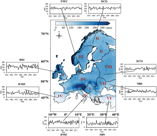
Table 1. The period, calibration model, number of chronologies, and some evaluation parameters used for reconstructions in the BRI.
Table 2. Brief information for reconstructions in the other five European regions. “Max” and “Min” refer to the maximum and minimum value of the parameters for each period, respectively.
Figure 3. Reconstructed hydroclimatic variations in six European regions.
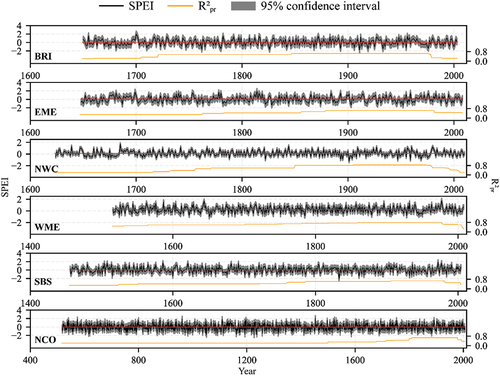
Figure 4. The 11-year sliding averages of the reconstructed hydroclimate series in six European regions over the past 500 years. Brown shading indicates a decreasing trend, while red shading indicates an increasing trend in the series during the specified period.
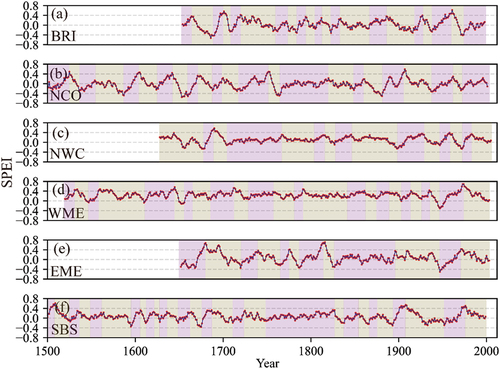
Figure 5. The 31-year sliding averages of the reconstructed hydroclimate series in six European regions over the past 500 years. Brown shading indicates a decreasing trend, while red shading indicates an increasing trend in the series during the specified period.
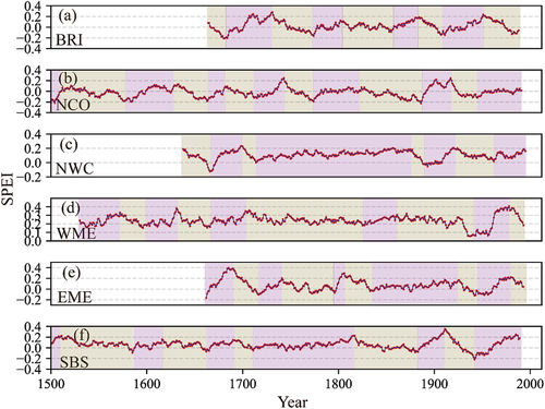
Figure 6. The and
of hydroclimatic variations in various European regions.
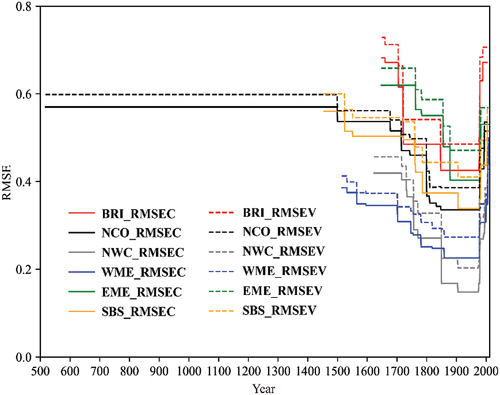
Figure 7. Comparison of reconstructed series in the BRI, WME, and SBS with previously reconstructed precipitation series from European regions, including (a) March-July precipitation (sums) in south-central England during 1650–2003 (Wilson et al., Citation2013) and (b) may-June precipitation (sums) in the northern Aegean region during 1450–1989 (Griggs et al., Citation2007).
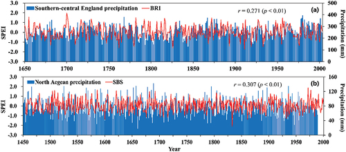
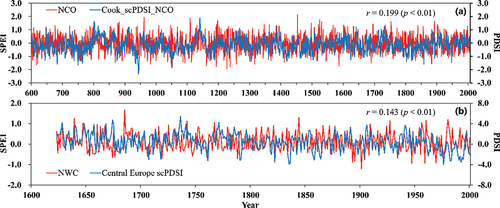
Figure 8. Comparison of reconstructions in the NCO and NWC with the previous reconstructed hydroclimate indicators in European regions, including (a) summer scPDSI of OWDA in the same NCO domain during 600–2006 (Cook et al., Citation2015), and (b) summer scPDSI in central Europe during 1623–2000 (Buntgen et al., Citation2021).
Supplemental Material
Download MS Word (42.2 KB)Data availability statement
The data that support the findings of this study are openly available in Science Data Bank at https://doi.org/10.57760/sciencedb.07215.