Sub-pixel building area mapping based on synthetic training data and regression-based unmixing using Sentinel-1 and -2 data

Figures & data

Table 1. Class hierarchy and number of pure reference samples. Bold: Target classes.

Level 1	Level 2	Number of Reference Samples
Impervious Surfaces	Building	147
	Non-Building	122
Woody Vegetation		90
Non-Woody Vegetation		277
Permanent Soil		166
Water		58

Figure 1. A: Direct and hierarchical regression-based unmixing approach with synthetically mixed training data from a pure surface feature library. STM = Spectral-temporal metrics, imp = impervious surfaces, b = building, nb = non-building impervious surfaces. Building area in (*) was validated. B: Example feature sets for two selected building and non-building impervious surfaces. TCG = Tasselled Cap Greenness, AVG = Average, STD = Standard Deviation, S1 VH AVG = Average Sentinel-1 VH Backscatter.

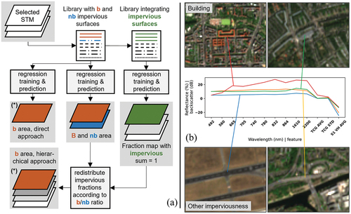
Figure 2. Density scatter plots of predicted and reference building area for the direct approach (blue) and the hierarchical approach (green) for 20 m (top), 50 m (centre) and 100 m (bottom) resolutions.

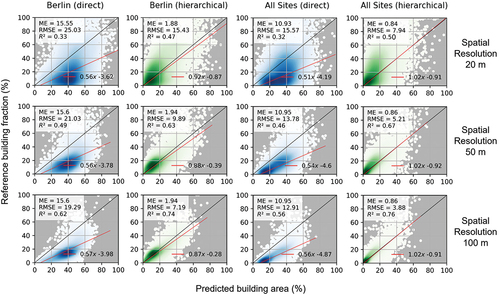
Figure 3. Density distribution of predicted building area at 10 m spatial resolution, split by pixels occupied by buildings (red) and non-building impervious surfaces (blue) in the three validated federal states.

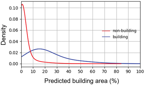
Figure 4. Predicted building area from the hierarchical approach at 100 m (left) and 10 m (centre) resolution, rasterized reference building footprints (right) for two sites in Berlin (top) and North Rhine-Westphalia (bottom). Scale valid for all subfigures.