Segmentation of high-voltage transmission wires from remote sensing images using U-Net with sample generation

Figures & data

Figure 1. Representative samples with different characteristics of transmission wires in high-resolution optical remote sensing images.

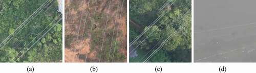
Figure 2. Flowchart of the Swin-Unet-M model for wire segmentation.

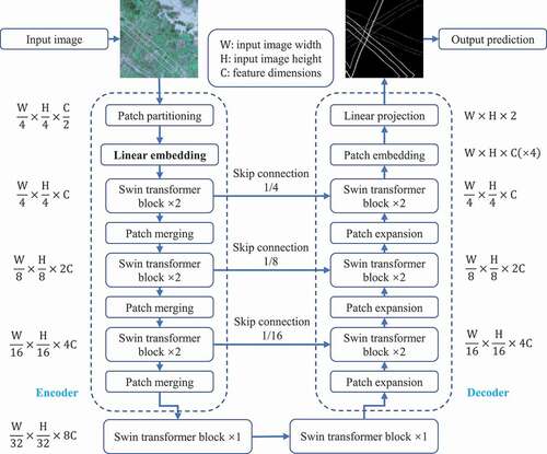
Table 1. The differences between Swin-Unet and Swin-Unet-M in ‘Linear Embedding’ module. Conv means the convolutional layer, $k$ means the kernel size, $s$ means the stride, $p$ means the padding size. Maxpool denotes the maxpooling layer. $B$ means the batch size. $C$ denotes the feature dimension ($C=96$ in this study).

	Linear embedding	Input shape	Output shape
Swin-Unet	Conv, $k=4$, $s=4$,$C$	$B\times 3\times 224\times 224$	$B\times C\times 56\times 56$
Proposed Swin-Unet-M (Refined)	Conv, $k=3$, $s=3$, $p=1$, $\frac{C}{2}$	$B\times 3\times 224\times 224$	$B\times \frac{C}{2}\times 224\times 224$
	Maxpool, $k=2$, $s=2$, $\frac{C}{2}$	$B\times \frac{C}{2}\times 224\times 224$	$B\times \frac{C}{2}\times 112\times 112$
	Conv, $k=3$, $s=3$, $p=1$,C	$B\times \frac{C}{2}\times 112\times 112$	$B\times C\times 112\times 112$
	Maxpool, $k=2$, $s=2$, C	$B\times C\times 112\times 112$	$B\times C\times 56\times 56$

Figure 3. Flow chart of the proposed synthetic wire sample generation.

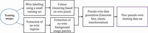
Figure 4. Visualization of segmentation results on synthetic test set. The images from left to right of each row are: original image, ground truth, the results obtained using FCN-Unet, Deeplab-Unet, PSP-Unet, Swin-Unet, and Swin-Unet-M.

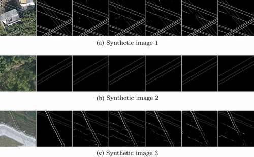
Table 2. Wire segmentation performance of three typical U-Net architectures with three different patch sizes (i.e., $64\times 64$, $128\times 128$, and $256\times 256$ pixels).

	$64\times 64$		$128\times 128$		$256\times 256$
	DSC	mIoU	DSC	mIoU	DSC	mIoU
FCN-Unet	$0.732\pm 0.007$	$0.578\pm 0.009$	$0.763\pm 0.008$	$0.617\pm 0.010$	$0.779\pm 0.009$	$0.638\pm 0.012$
Deeplab-Unet	$0.727\pm 0.007$	$0.572\pm 0.009$	$0.761\pm 0.005$	$0.615\pm 0.006$	$0.775\pm 0.005$	$0.633\pm 0.007$
PSP-Unet	$0.734\pm 0.006$	$0.581\pm 0.008$	$0.761\pm 0.005$	$0.615\pm 0.007$	$0.774\pm 0.004$	$0.631\pm 0.006$

Table 3. Wire segmentation performance of the Swin-Unet and Swin-Unet-M with different learning rates (LR). The bold numbers mean the best result.

	$LR=0.05$		$LR=0.1$		$LR=0.2$
	DSC	mIoU	DSC	mIoU	DSC	mIoU
Swin-Unet	$0.838\pm 0.008$	$0.722\pm 0.012$	$0.828\pm 0.042$	$0.709\pm 0.058$	$0.737\pm 0.178$	$0.610\pm 0.190$
Swin-Unet-M	$0.834\pm 0.007$	$0.716\pm 0.010$	$0.855\pm 0.004$	$0.746\pm 0.007$	$\mathbf{0}.\mathbf{859}\pm \mathbf{0}.\mathbf{007}$	$\mathbf{0}.\mathbf{754}\pm \mathbf{0}.\mathbf{012}$

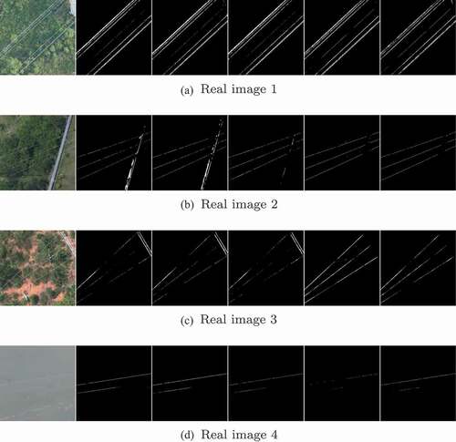
Figure 5. Visualization of segmentation results on four real images. The images from left to right of each row are: original image and the results obtained using FCN-Unet, Deeplab-Unet, PSP-Unet, Swin-Unet and the proposed Swin-Unet-M, respectively.