Effects of herbicide application to control sward composition in different management variants

Figures & data

Table 1. Experimental factors and treatment levels of the GrassMan experiment

Factor	Level	Acronym	Time scope
Sward type	1.1 Untreated control sward	Co	One herbicide application
	1.2 Dicots reduced	−Dic
	1.3 Monocots reduced	−Mon
Utilization	2.1 Cut once (July)	1	Continuous management
	2.2 Cut three times (May, July, September)	3
Fertilization	3.1 No fertilization	x
	3.2 180/30/100 kg N/P/K ha^−1 yr^−1a	NPK
Notes: The acronyms of the different treatments are generated by the combination of the factor level abbreviations in the order sward-utilization-fertilization, e.g. –Dic1x = dicot-reduced sward, cut once, no fertilization. The four combinations of utilization and fertilization are referred to as management categories in the text.
^aN fertilizer: calcium ammonium nitrate N27, P&K fertilizer: Thomaskali® (8% P2O5, 15% K2O, 20% CaO).

Table 2. Relative change of degree of presence of the 20 most frequent species in 9 m² before (June 2008) and after (May, August 2009) the herbicide application within the three sward types

		Relative change
Overall degree of presence in 9 m^2 (%)		(± % of presence in June 2008)
	June 2008	May 2009			August 2009
	All plots	Co	−Dic	−Mon	Co	−Dic	−Mon
Poa pratensis ag.	98.6	0	−12.5	−8.3	−2.1	−6.2	−4.2
Lolium perenne	97.9	2.2	0	0	0	−4.2	−19.1
Festuca rubra	95.8	−2.1	0	2.1	−12.8	−10.9	−2.2
Dactylis glomerata	70.1	20.6	23.6	15.1	20.6	11.9	0
Poa annua	29.9	−84.5	−71.6	−93.7	−100	−92.8	−93.7
Deschampsia cespitosa	28.5	−6.0	22.9	−16.8	−12.3	0	8.4
Holcus mollis	27.1	−24.9	33.0	−14.4	−37.5	−11.2	0
Ranunculus repens	100	0	−2.1	0	0	0	0
Trifolium repens	100	0	−89.6	0	0	−68.7	0
Veronica chamaedrys	99.3	0	−2.1	−2.1	0	2.1	−2.1
Cerastium holosteoides	98.6	−4.2	−87.5	2.1	−55.3	−83.3	−19.1
Rumex acetosa	98.6	2.2	−2.1	0	4.4	0	0
Stellaria graminea	95.1	−4.2	−95.6	4.5	−34	−69.5	−13.6
Taraxacum Sec. Ruderalia	73.6	14.8	5.6	30.5	32.5	22.3	30.5
Achillea millefolium	66.7	13.3	−56.6	−2.8	10.1	−13.3	8.4
Cardamine pratensis	53.5	29.5	−34.7	41.6	−29.7	−65.3	−54.2
Cirsium arvense	34.0	−33.3	−64.7	0	−14.4	−23.4	9.2
Rumex obtusifolius	27.8	−33.2	−33.2	−6.0	−24.8	−8.4	−24.9
Note: Means over management categories.

Table 3. Importance of the experimental factors in explaining the differences in annual yield 2009

Factors	df	Sum^2	Mean^2	F value	P (>F)	Percent of variance explained
Sward type	2	135.9	67.9	0.4546	0.637	0.28
Fertilization	1	27670.1	27670.1	185.1709	<0.001	58.5
Utilization	1	5859.4	5859.4	39.2114	<0.001	10.4
Fertilization × Utilization	1	4825.1	4825.1	32.2903	<0.001	8.6
Notes: ANOVA including spatial effects (row + block). Response variable square root transformed.

Table 4. Proportion of variation in single and total yields 2008–2009 explained by the experimental factors (%)

	June 2008	Oct 2008	May 2009	July 2009	September 2009	Total 2009	July 1 cut	July 3 cuts
Sward type	1.7	26.6***	7.2	1.1	0.4	0.2	1.7	2.1
Utilization	0.5			37.4***		58.5***
Fertilization	0	23.1***	32.0***	39.3***	77.7***	10.4***	50.9***	77.3***
Use × Fert				1.0′		8.6***
Sw × Fert								2.7*
Notes: June 2008 is the baseline yield without any experimental treatments. ANOVA based on gls estimation allowing for different variances per utilization (June 2008), per fertilization level (July 2009, July 1 cut) or per sward type (September 2009) or based on linear models with transformation of the response variable. Response variable raised to the power of 0.25 (October 2008, May 2009), or 0.5 (July 3 cuts, total 2009). ***P < 0.001, *P < 0.

Figure 1. Relationships between total yield 2009 and proportions of grasses (a), forbs (b) and legumes (c) under the four management regimes (legend: middle right). None of the correlations between yield and independent variable within one management category were significant. For abbreviations of experimental treatments please refer to Table 1.

Figure 2. Yield May 2009 dependent on proportion of tall grasses (a) and proportion of small species (b) grouped by fertilization level (with regression lines). The corresponding linear model includes a significant interaction between nutrients and tall grasses (P = 0.032) and nutrients and small species (P = 0.017), response variable untransformed.

Figure 3. Box and whisker plots showing the four quartiles, the median (calculation of outliers by the default method in R) and the means, denoted by small squares, of selected forage quality characteristics in the six different sward type × fertilization level combinations at each of the three harvests. Second cut (July) of the three cut regime not presented. Asterisks denote significant differences from the control sward of the same fertilization level (***P < 0.001, **P < 0.01, *P < 0.05, (*)P = 0.0506). Linear contrasts in linear models; either models with different variances per fertilization level (graphs (c), (k)) or sward type (graph (f)) or response variable either square root (graph (h)) or not transformed (all others). For abbreviations of experimental treatments please refer to Table 1.

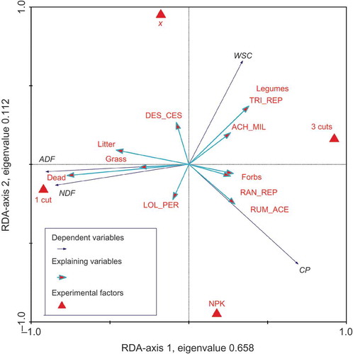
Figure 4. Ordination diagram of a redundancy analysis (RDA) with forage quality characteristics (contents of CP, WSC, ADF, NDF in 2009, untransformed) as dependent variables and the experimental factors utilization and fertilization (cf. Table 1) and vegetation characteristics (instead of sward types) as explaining variables. Quality characteristics of the three-cut variant are averaged across harvest dates. Explaining variables with a correlation coefficient with the first and second ordination axis <–0.2 and >0.2 are included.