Aquatic faunal abundance and diversity in relation to synthetic and natural pesticide applications in rice fields of Central Thailand

Figures & data

Figure 1. Data  variation of plankton variables (taxonomic and functional groups) as explained by independent predictors (biophysical, farm, and pesticide variables). The numbers indicate whether the tested variables are from the first (1) or from the second (2) survey. Inserted triangles indicate a significant change of the variables from the first to the second survey (as determined from paired T-tests or Mann–Whitney tests), where ▲ indicates significantly higher and ▼ lower levels at the respective sampling time; ◊ indicates no significant change. The significance levels of the changes are indicated by the darkness of the triangles, from ▲ (p < 0.0005), ▲ (p < 0.005), to ▲ (p < 0.05). The inserted numbers represent average organism counts per liter, respectively mass indices (xⁱ; ~volume in mm³ per liter). The arrows indicate the predictor variables (at the start of the arrows) which were significant in the models in order to explain the dependent variables (at the end of the arrows). The arrows may or may not imply causality. White arrows represent positive and black arrows negative correlations. The thickness of the arrows indicates the significance level of the correlation from the thickest (p < 0.0005), medium (p < 0.005), to the thinnest (p < 0.05). ‘Farm type’ and ‘Province’ refer to ‘organic’ farms and ‘Ayutthaya Province’, respectively. Correlations among plankton variables (all positive) are indicated by light connecting lines with thicknesses corresponding to significances. I. = index; cumul. = cumulative; plankt. = plankton; H = height; D = density; N = nitrogen content; dist. = distance; Cyperm. = cypermethrin.

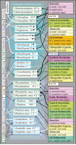
Figure 2. Data  variation of invertebrate variables (only arthropods; taxonomic and functional groups) as explained by independent predictors (plankton, biophysical, farm, and pesticide variables). Refer to legend of Figure 1 for an explanation of the arrows, numbering, and triangles. The figures represent (a) average organism counts in all net samples per farm, (b) average total mass indices (xⁱ; ~volume in mm³ in all net samples per farm), (c) average organism mass indices (xⁱ; ~mm³), (d) average number of species, and average levels of biodiversity as described by (e) the Shannon–Weiner index, and (f) the Shannon Evenness index. Correlations between herbivore and predator group variables (all positive) are indicated by light connecting lines with thicknesses corresponding to significances. I. = index; cumul. = cumulative; H = height; D = density; fish ct = fish counts; dist. = distance; spp = species; org. = organism; even. = evenness; OC = organic carbon content; GAS = golden apple snail; Cyperm. = cypermethrin.

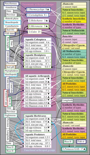
Figure 3. Principal components analysis (PCA) plot illustrating the multivariate correlations of selected plankton, invertebrate, fish, and waterfowl variables, as well as pesticide and biophysical variables (also including the factors ‘province’ and ‘farm type’). The pesticide variables refer to ‘seasonal toxic input’ (crop) or ‘cumulative toxic input’ (cumul.). The interval data were all transformed to a normal distribution. The PCA eigenvalues of the first and second components were 6.92 and 5.10, respectively. GAS = golden apple snail; spp = species; richn. = richness; Sh. = Shannon.

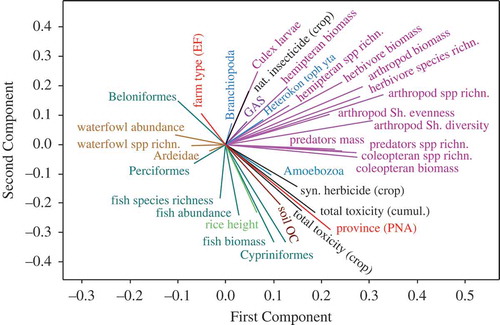
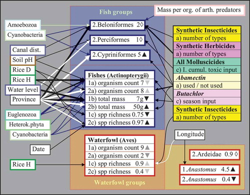
Figure 4. Data  variation of fish and waterfowl variables (vertebrates) as explained by independent predictors (invertebrate, plankton, biophysical, farm, and pesticide variables). Refer to legend of Figure 1 for an explanation of the arrows, numbering, and triangles. The figures represent (a) average organism counts during standardized observations per farm, (b) average total mass indices (in grams), and (c) average number of species. Correlations between fish and invertebrate or plankton variables are indicated by connecting lines with thicknesses corresponding to significances, dark lines indicating negative and light lines indicating positive correlations. arth. = arthropod; other abbreviations cf. Figure 2.