Figures & data
Figure 1. Map of Central Thailand showing the location of the two study sites in Bang Sai district, Phranakhon Si Ayutthaya (PNA) province, and in Muang Ang Tong district, Ang Tong (AT) province.
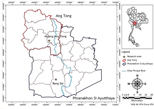
Figure 2. Average monthly temperature (daily maximum and minimum) for Phranakhon Si Ayutthaya (PNA), and average monthly rainfall for the years 2001–2011 (mean) and for 2011 for Ang Tong (AT) and Ayutthaya provinces.
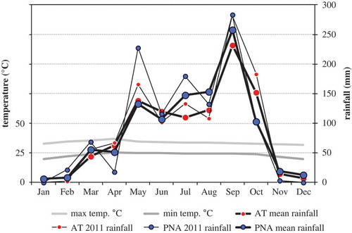
Figure 3. Data variation of respondent and land possession variables as explained by independent predictors (farm variables). The arrows indicate the predictor variables (at the start of the arrows) that were significant in the models to explain the dependent variables (at the end of the arrows). The arrows may or may not imply causality. White arrows represent positive and black arrows represent negative correlations (in multivariate models). The thickness of the arrows indicates the significance level of the correlation from the thickest (p < .0005), medium (p < .005), to the thinnest (p < .05). ‘Farm type’ and ‘province’ refer to ‘organic, extensively managed farms’ (EF) and ‘Ayutthaya province’ (PNA), respectively.
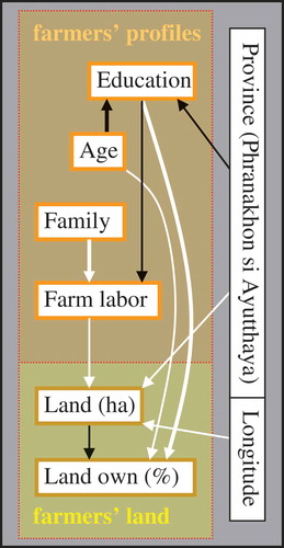
Table 1. The average number (± standard deviation) of different synthetic and natural pesticides used in the two provinces on intensive (IF) and ecologically oriented (EF) farms.
Figure 4. Cumulative density function (CDF, including a lognormal fit) of the ‘index of seasonal toxic input’ on the farmers’ fields of the two provinces (Ayutthaya and Ang Tong) and farm types (organic and intensive). The index may be interpreted as a maximum number of rats (in thousands) that could in theory be killed if the total volume of all pesticides spread seasonally on a hectare of rice field were instead to be fed to rats orally. The three parameters for each of the four lognormal distribution models are shown in the inset table.
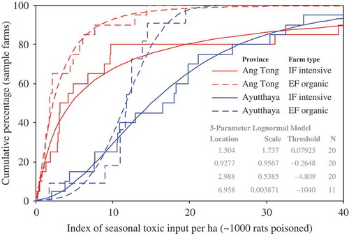
Figure 5. Cumulative density function (CDF, including a lognormal fit) of the ‘index of cumulative toxic input’ on the farmers’ fields of the two provinces (Ayutthaya and Ang Tong) and farm types (organic and intensive). The index may be interpreted as an approximate maximum number of rats (in thousands) that could in theory be killed if the total volume of all pesticides spread in cumulative total (i.e. since the introduction of the respective pesticides) on a hectare of rice field were instead to be fed to rats orally. The three parameters for each of the four lognormal distribution models are shown in the inset table.
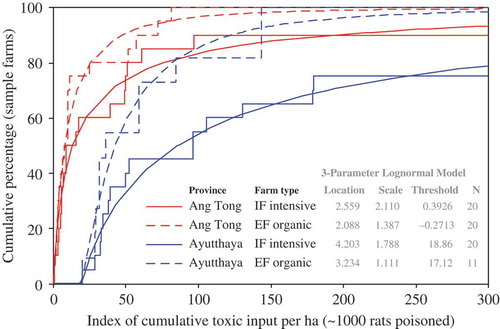
Figure 6. Data variation of various pesticide variables (uses, application levels, and indices of toxic input) as explained by independent predictors (farm, respondent, and land possession variables). Refer to legend of for an explanation of the arrows. For the major pesticide groups (overall, and synthetic/natural insecticides, herbicides, and molluscicides), the percentage of users is indicated (in brackets) as well as the summary statistics on the ‘number of pesticide types’ (average ± standard deviation) and indices of toxic input (the median index (excluding ‘0’) and the percentage contribution of the overall toxic input of the respective group in relation to the total toxic input of all pesticides in the fields) is indicated. For the four most commonly used synthetic pesticide types (i.e. chlorpyrifos + cypermethrin, abamectin, butachlor, clomazone + propanil), the toxicity is indicated (the 50% lethal dose (LD50) in grams needed to kill 1 kg of rats), as well as the averages (± standard deviations; excluding ‘0’) of the doses (in cc/ha) used per application, per season, and for the entire period since the chemical was introduced (cumulative input) are indicated. The average (± standard deviation) of the dose used per application is also indicated for tea seed powder (I. = index; cumul. = cumulative).
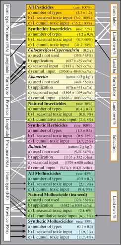
Figure 7. Principal component analysis loading plot illustrating the multivariate correlations of different selected pesticide, soil and rice growth variables, also including the factors ‘province’ and ‘farm type’ and the field variables ‘water depth’ and ‘distance to irrigation canals’. The pesticide variables refer to ‘seasonal toxic input’ (crop) or ‘cumulative toxic input’ (cumul.). Rice density and growth are shown during the wet (WS) and dry (DS) seasons (DS is based on 40 true data points and 31 ‘dummy’ data points, i.e. averages). The interval data were all transformed to a normal distribution. The PCA eigenvalues of the first and second components were 7.45 and 3.01, respectively. (syn. = synthetic; nat. = natural; cumul. = cumulative; cyperm. = cypermethrin; DS = dry season; WS = wet season; OC = organic carbon content; N = nitrogen content).
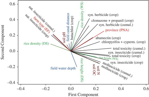
Figure 8. Scatterplot showing the increase in soil organic matter content as a function of the ‘index of seasonal toxic input’ of all the pesticides. The equation and statistics of the simple regression model are also provided.
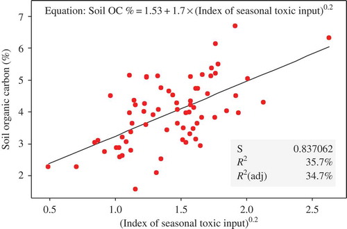
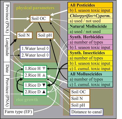
Figure 9. Data variation of biophysical field variables – water levels, soil organic matter and nitrogen contents, soil pH levels, and rice plant sizes H (height in cm) and densities D (plant counts per m2) – as explained by independent predictors (farm and pesticide variables). Refer to legend of for an explanation of the arrows. The numbers indicate whether the tested variables are from the first (1) or from the second (2) survey. Inserted triangles indicate a significant change of the variables from the first to the second survey (as determined from paired t-tests or Mann–Whitney tests), where ▲ indicates significantly higher and ▼ indicates lower levels at the respective sampling time; ◊ indicates no significant change. The significance levels of the changes are indicated by the darkness of the triangles, from ▲ (p < .0005), ▲ (p < .005), to ▲ (p < .05). (I. = index; cumul. = cumulative; H = height; D = density; OC = organic carbon content; N = nitrogen content; Cyperm. = cypermethrin).