1,558
Views
8
CrossRef citations to date
0
Altmetric
Primary Research

Neuronal spike-train responses in the presence of threshold noise

, , , &
Pages 91-105 | Received 30 Apr 2010, Accepted 30 Jun 2010, Published online: 26 Mar 2012

Figures & data

Figure 1. The probability of firing in a model with Gaussian threshold noise. Here V th=−40 mV and σ=4 mV−1 (black), σ=3 mV−1 (red), σ=2 mV−1 (green), σ=1 mV−1 (blue) and σ=0.5 mV−1 (magenta).
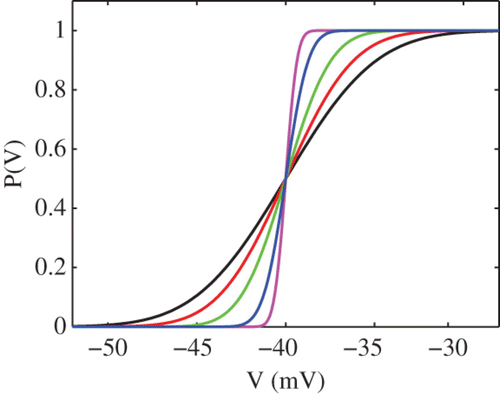
Figure 1. The probability of firing in a model with Gaussian threshold noise. Here V th=−40 mV and σ=4 mV−1 (black), σ=3 mV−1 (red), σ=2 mV−1 (green), σ=1 mV−1 (blue) and σ=0.5 mV−1 (magenta).

Figure 2. Loss of synchrony with increasing noise strength in a network of 1000 uncoupled leaky IF neurons for different values of the ratio of the driving frequency to the natural frequency of the neuron, sω ≡ ω/ω0, and the amplitude of forcing, a. Parameter values are (left) sω=1.1, a=1, (middle) sω=2.2, a=2, (right) sω=3.1, a=1.5. Other parameter values are η=2 ms, I 0=2.4, V L=V R=−60 mV, V th=−40 mV and τ=10 ms.

Figure 2. Loss of synchrony with increasing noise strength in a network of 1000 uncoupled leaky IF neurons for different values of the ratio of the driving frequency to the natural frequency of the neuron, sω ≡ ω/ω0, and the amplitude of forcing, a. Parameter values are (left) sω=1.1, a=1, (middle) sω=2.2, a=2, (right) sω=3.1, a=1.5. Other parameter values are η=2 ms, I 0=2.4, V L=V R=−60 mV, V th=−40 mV and τ=10 ms.

Figure 3. A plot of the amplitude of the population response function |δ rI|/r 0 for a leaky integrator network as a function of sω≡ω/ω0 for σ=0.01 (black), σ=0.1 (green), σ=0.15 (blue), σ=0.2 (red) and σ=0.25 (magenta). The response function becomes progressively flatter and resonances are abolished as the blow up around sω=1 on the right illustrates. Other parameter values are V L=V R=−60 mV, V th=−40 mV, τ=10 ms and I 0=2.3.
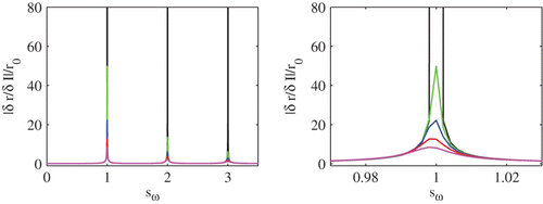
Figure 3. A plot of the amplitude of the population response function |δ r/δ I|/r 0 for a leaky integrator network as a function of sω≡ω/ω0 for σ=0.01 (black), σ=0.1 (green), σ=0.15 (blue), σ=0.2 (red) and σ=0.25 (magenta). The response function becomes progressively flatter and resonances are abolished as the blow up around sω=1 on the right illustrates. Other parameter values are V L=V R=−60 mV, V th=−40 mV, τ=10 ms and I 0=2.3.

Figure 4. Network rate r (dots) for σ=0.001 mV (left) and σ=5.5 mV (right) in the 1:1 case for sω=1.1 and a=1. The solid black line in the right panel corresponds to the oscillating input signal. Other parameter values are η=2 ms, I 0=2.4, V L=V R=−60 mV, V th=−40 mV and τ=10 ms.
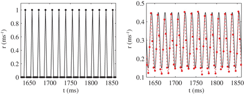
Figure 4. Network rate r (dots) for σ=0.001 mV (left) and σ=5.5 mV (right) in the 1:1 case for sω=1.1 and a=1. The solid black line in the right panel corresponds to the oscillating input signal. Other parameter values are η=2 ms, I 0=2.4, V L=V R=−60 mV, V th=−40 mV and τ=10 ms.

Figure 5. Left: Membrane potential (solid black line) and threshold (dotted black line) for different sinusoidal drive. Right: ISI distribution corresponding to the trajectories on the left; analytical results (solid black line) and histograms from direct numerical simulations (grey bars). Parameter values are from top to bottom η=2 ms, σ=0.2, sω=1.2, a=1, I 0=2.3; η=2 ms, σ=0.2, sω=2.2, a=2, I 0=2.3; η=2 ms, σ=0.1, sω=1.2, a=1, I 0=2.3; η=2 ms, σ=0.2, sω=1.2, a=1, I 0=2.4. Other parameter values are V L=V R=−60 mV, V th=−40 mV and τ=10 ms.
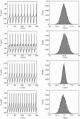
Figure 5. Left: Membrane potential (solid black line) and threshold (dotted black line) for different sinusoidal drive. Right: ISI distribution corresponding to the trajectories on the left; analytical results (solid black line) and histograms from direct numerical simulations (grey bars). Parameter values are from top to bottom η=2 ms, σ=0.2, sω=1.2, a=1, I 0=2.3; η=2 ms, σ=0.2, sω=2.2, a=2, I 0=2.3; η=2 ms, σ=0.1, sω=1.2, a=1, I 0=2.3; η=2 ms, σ=0.2, sω=1.2, a=1, I 0=2.4. Other parameter values are V L=V R=−60 mV, V th=−40 mV and τ=10 ms.

Figure 6. ISI distribution for different noise strengths: σ=0.1 (top left), σ=0.5 (top right), σ=1 (bottom left), σ=2 (bottom right). The deterministic dynamics shows a 1:4 mode-locked state. Other parameter values are η=2 ms, sω=4.1, a v =2.25, I 0=2.4, V L=V R=−60 mV, V th=−40 mV and τ=10 ms.
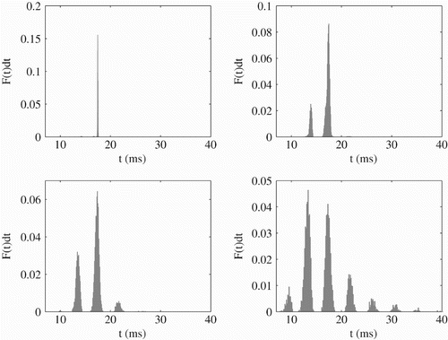
Figure 6. ISI distribution for different noise strengths: σ=0.1 (top left), σ=0.5 (top right), σ=1 (bottom left), σ=2 (bottom right). The deterministic dynamics shows a 1:4 mode-locked state. Other parameter values are η=2 ms, sω=4.1, a v =2.25, I 0=2.4, V L=V R=−60 mV, V th=−40 mV and τ=10 ms.

Figure 7. ISI distribution when the deterministic dynamics shows a 2:1 mode-locked state. Parameter values are σ=0.5, sω=0.5, a=1, η=2 ms, I 0=2.4, V L=V R=−60 mV, V th=−40 mV and τ=10 ms.
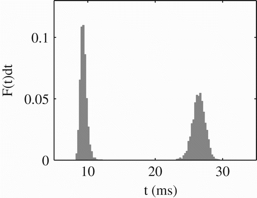
Figure 7. ISI distribution when the deterministic dynamics shows a 2:1 mode-locked state. Parameter values are σ=0.5, sω=0.5, a=1, η=2 ms, I 0=2.4, V L=V R=−60 mV, V th=−40 mV and τ=10 ms.

Figure 8. Plots of the Liapunov exponent in the (a, sω) plane showing Arnol'd tongues for σ=0, 0.5, 1, 1.5, 2, 2.5 parameter values are η=2 ms, I 0=2.3, V L=V R=−60 mV, V th=−40 mV and τ=10 ms.
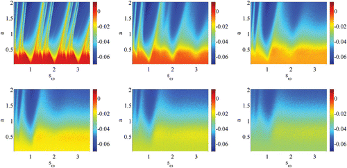
Figure 8. Plots of the Liapunov exponent in the (a, sω) plane showing Arnol'd tongues for σ=0, 0.5, 1, 1.5, 2, 2.5 parameter values are η=2 ms, I 0=2.3, V L=V R=−60 mV, V th=−40 mV and τ=10 ms.

Figure 9. A-C. ISI scattergrams of the responses of a VCN chopper unit to amplitude modulated tones. The tone was 3 s long, with a frequency the same as the characteristic frequency of the unit, 50 dB above the CF threshold. AM depth was 100% and frequency was as indicated. D-F. The responses of a stochastic-threshold IF model fitted to the data. The model parameters were: sinuisodal input: a=0.7, I 0=1.5 mV, threshold noise: σ=2.7, η=0.75 ms, IF parameters: τ=3.18 ms, V L=V R=−60 mV, V th=−42 mV. G. An example of the evolution of the membrane potential of the model (blue) for the 50 Hz modulation rate, the stochastic threshold (green) and the modulated input on an arbitrary scale.
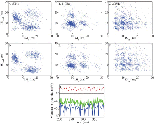
Figure 9. A-C. ISI scattergrams of the responses of a VCN chopper unit to amplitude modulated tones. The tone was 3 s long, with a frequency the same as the characteristic frequency of the unit, 50 dB above the CF threshold. AM depth was 100% and frequency was as indicated. D-F. The responses of a stochastic-threshold IF model fitted to the data. The model parameters were: sinuisodal input: a=0.7, I 0=1.5 mV, threshold noise: σ=2.7, η=0.75 ms, IF parameters: τ=3.18 ms, V L=V R=−60 mV, V th=−42 mV. G. An example of the evolution of the membrane potential of the model (blue) for the 50 Hz modulation rate, the stochastic threshold (green) and the modulated input on an arbitrary scale.