Influence of the genomic sequence on the primary structure of chromatin

Figures & data

Figure 1. In vivo experimental nucleosome mapping along S. cerevisiae chromosomes obtained by Lee et al. (2007) (MNase-chip). Nucleosome occupancy profile (, where Y(s)=log ₂(P(s))) along a 10 kpb fragment of chromosomes 2 (a), 7 (b), 12 (c) and 14 (d). Symbols indicate regulatory sites: Transcription Start Sites (TSS, red dots), Transcription Termination Sites (TTS, pink circles) and Transcription Factors Binding Sites (TFBS, black triangles).

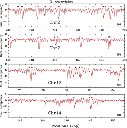
Figure 6. In vivo nucleosome (non-normalized) occupancy profile P(s) along chromosome 2 of the human genome (Schones et al. 2008). (a) P(s) versus s along a 100 kbp fragment as obtained from the 5′ and 3′ ends tag profiles (see Zhang and Pugh 2011). (b) Zoom on a 10 kbp region.

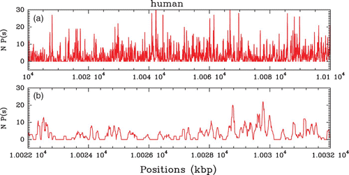
Figure 2. In vivo nucleosome occupancy profile δ Y(s) (see Figure 1) along a 10 kbp fragment of chromosome 3 (a), 2 (b) and 2 (c) of S. cerevisiae. Comparison of Lee et al. (2007) MNase-chip data (red) with (a) Yuan et al. (2005) MNase-chip data (green), (b) Whitehouse et al. (2007) MNase-chip data (blue) and (c) Kaplan et al. (2009) MNase-seq data (violet). The symbols have the same meaning as in Figure 1. In (b), the Whitehouse et al. data correspond to a detrended hybridation profile: with a∼200 bp. For the sake of comparison, we have applied the same detrending procedure to the Lee et al. data in (b).

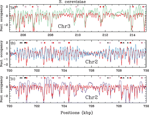
Figure 3. (a) In vivo nucleosome occupancy profile δ Y(s) (see Figure 1) along a 650 kbp fragment of chromosome C of S. kluyveri. MNase-seq data of Tsankov et al. (2010). (b) (resp. (c)), zoom on the 50 kbp region indicated in (a) by the red (resp. orange) colored segment, that corresponds to a high (resp. low) (G+C) content region, namely 52% (resp. 40%) as compared to the mean genome value (G+ C);=40%.

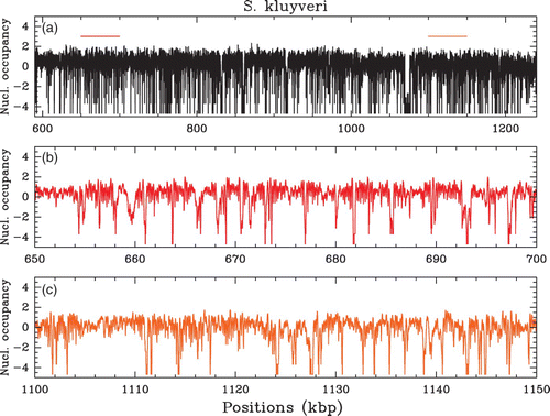
Figure 4. In vivo nucleosome occupancy profile δ Y(s) (see Figure 1) along a 10 kbp fragment of chromosome 2 of S. pombe. (a) MNase-chip data of Lantermann et al. (2010): comparison between the WT (red) and the mit1-mutant (green). (b) Comparison between WT MNase-chip data of Lantermann et al. (red, see (a)) and the MNase-seq data of Tsankov et al. (2011) (cyan).

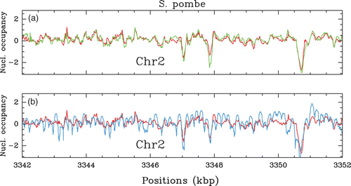
Figure 5. In vivo nucleosome occupancy profile δ Y(s) (see Figure 1) along chromosome 2 of C. elegans (Valouev et al. 2008). (a) δ Y(s) versus s (green) along a 100 kbp fragment as obtained from the 5′ and 3′ ends’ tag profiles (black, see Zhang and Pugh 2011). (b) Zoom on a 10 kbp region.

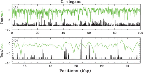
Figure 7. Histograms of nucleosome occupation Y(s) values centered on their typical values (i.e. the maximum of the histogram is positioned at zero) for different sets of in vivo data. (a) S. cerevisiae MNase-chip data of Lee et al. (2007). (b) S. cerevisiae MNase-seq data of Shivaswamy et al. (2008) (green) and of Kaplan et al. (2009) (violet) as compared to S. pombe MNase-seq data of Tsankov et al. (2011) (cyan). (c) S. pombe MNase-chip data of Lantermann et al. (2010): WT (red) and Mit1 mutant (green); the dashed curve corresponds to the S. cerevisiae Lee et al. data shown in (a). (d) C. elegans (green) and human (red) MNase-seq data of Valouev et al. (2008) and Schones et al. (2008), respectively.

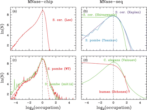
Figure 8. (a) Auto-correlation function C(Δ s)=⟨ δ Y(s) δ Y(s+Δ s) ⟩ versus Δ s. (b) Corresponding power spectrum. The different colors correspond to the following S. cerevisiae data sets: MNase-chip data of Lee et al. (2007) (red) and of Whitehouse et al. (2007) (blue); MNase-seq ‘tag’ data of Shivaswamy et al. (2008) (green).

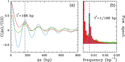
Figure 9. Histograms of local NRL values computed from different nucleosome occupancy data sets. The different colors correspond to the following data: S. cerevisiae MNase-chip data of Lee et al. (2007) (red); S. pombe MNase-seq data of Tsankov et al. (2011) (cyan); C. elegans MNase-seq data of Valouev et al. (2008) (green). (Inset) Comparison betwen the histograms of the S. cerevisiae NRLs (Lee et al. 2007) (red) and of S. kluyveri NRLs (Tsankov et al. 2010) (orange).

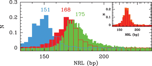
Figure 17. Gradual increase of NRL by histone H1. (a) Chromatin was assembled in histone depleted embryo extracts complemented with core histones and the indicated amounts of histone H1. (b) Plot profile of the first lane of each MNase digestion in (a). Peaks of mono- (M), di- (D) and tri-nucleosomes (T) are indicated. Adapted from Blank and Becker (1995).

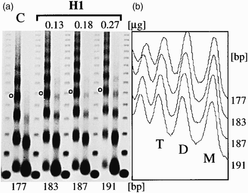
Figure 10. Nucleosome occupancy profile (, where Y(s)=log ₂(P(s))) along a 15 kpb long fragment of S. cerevisiae chromosomes 12: (a) in vivo MNase-chip data of Lee et al. (2007) (red) and in vivo MNase-seq data of Kaplan et al. (2009) (violet); (b) in vitro MNase-seq data of Kaplan et al. (2009) (orange); (c) corresponding histograms of Y(s) values centered on their typical values; (d) auto-correlation functions C(Δ s)=⟨ δ Y(s) δ Y(s+Δ s) ⟩.

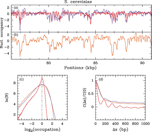
Figure 11. Grand canonical model of nucleosome assembly: bulk histones (green) may adsorb on or desorb from DNA (arrows). Barriers, such as transcription factors or other DNA binding proteins (red) can hinder nucleosome formation. The dynamics is controlled by a thermal bath (kT), the chemical potential of the histone reservoir (μ), the nucleosome–nucleosome interaction (V(r _i , r _j )) and the non-homogeneous adsorbing potential E(s). When no tridimensional degree of freedom is considered, the system reduces to a one-dimensional Tonks–Takahashi fluid of hard-rods of hard core size the DNA wrapping length l (Tonks 1936; Takahashi 1942).

Figure 12. Illustration of the Vanderlick et al. exact solution (blue) of the Percus equation [Equation (16)]. The energy landscape (E(s)) used for the computation is shown in green. (a) f(s) ‘forward’ function; (b) b(s) ‘backward’ function; (c) the resulting density ρ(s)=f(s)b(s). Model parameters: potential wall amplitude=+30 kT, μ=+3 kT.

Figure 13. Hard-rod occupancy profiles P(s) in a non-uniform energy landscape made of discrete energy barriers and traps and bounded by two infinite walls (black). The Percus equation (16) was solved using the Vanderlick et al. integration scheme (subsection ‘Resolution of the Percus equation: the exact solution of Vanderlick et al.’) at low chemical potential μ=−6 kT (orange) and high chemical potential μ=−1 kT (red). The occupancy values ρ _b l=0.19 (resp. ρ _b l=0.74) correspond to the bulk occupancy of the uniform system at μ=−6 kT (resp. μ=−1 kT ) (see Figure 14).

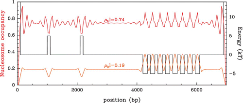
Figure 14. Occupancy (ρ l) of hard rods in a homogeneous energy landscape E(s)=E _o , as a function of the residual chemical potential μ˜=μ−E _o . Theoretical curves obtained from Equation (14) (red, infinite size system) and from Vanderlick numerical method (blue, large but finite size system). The dots indicate the bulk occupancy values for the chemical potential values used in Figure 13: μ˜=−6 kT (orange dot) and μ˜=−1 kT (red dot).

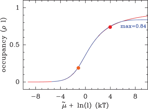
Figure 27. Energy landscape E(s) computed with the following parameter values: and l _w =125 bp along 10 kbp fragments of the chromosome 1 of C. elegans (green). Disordered patterns (regions D ₁, D ₂ and D ₃) are alternating with regular patterns, either quasi-flat (regions F ₁, F ₂, F ₃, F ₄ and F ₅) or periodic with periodic stretches of barriers/wells (R ₁ and R ₂). In red are reported the experimental occupancy data δ Y(s) of Valouev et al. (2008).

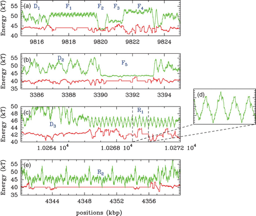
Figure 15. Evolution of the pair function g(r) [Equation (44)] with the residual chemical potential μ˜. Black and red curves correspond to a chemical potential μ˜=−5 kT and+5 kT respectively. Gray curves correspond to intermediate values of μ˜. The inter-particle distance r=|s ₁−s ₂| is expressed in l units.

Figure 16. (a) Pair function g(r) of a dense (uniform, E(s)=E _o =c ^ste ) hard-rod fluid. The residual chemical potential is μ˜=0 which gives a bulk density ρ _b l=0.78. The statistical ordering of this dense phase is characterized by the period and the range of the oscillating pattern: (inset) ln(g _m (i)l−1) as a function of p _m (i)−l, where g _m (i) is the value of the pair function at the ith extremum and p _m (i) is the position of the ith extremum: maximum (red points) and minimum (green points) of the pair function. The linear regression gives a slope−λ=−1.9 l, with λ defining the damping length. (b) Position p _m (i) of the ith maxima (red) or minima (green) as a function of i. The linear regression gives the mean period of the oscillations l*=1.2 l. (c) Evolution of the ordering range λ (black) and the mean period l* (red) as a function of the chemical potential μ˜. Both lengths are measured as explained in (a) and (b). In blue is reported the mean inter-nucleosome distance as a function of μ˜.

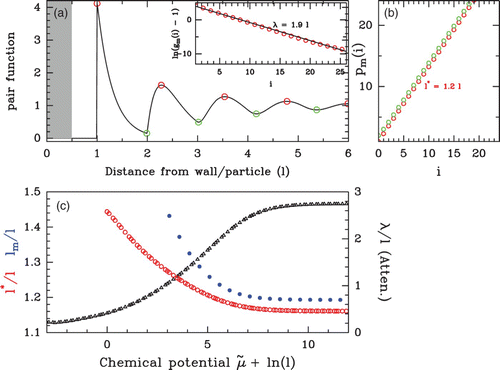
Figure 18. Evolution of the density profile ρ(s) with the chemical potential μ˜ from μ˜=−5 kT (black) to+5 kT (red). Statistical confinement near an infinite wall (a) and in between two infinite energy barriers (b).

Figure 19. (a) Aggregation of nucleosome signals around CTCF sites from the experiment of Fu et al. (2008). The coordinate origin is set to the 5′ end position of the 20 bp-long CTCF sites. Schematic arrangement of nucleosomes (blue ovals) around a CTCF binding site (orange rectangle). Blue arrows indicate sequence tags on the same strand as the CTCF site (nucleosome 5′ extremity) and orange arrows indicate opposite-strand tags (nucleosome 3′ extremity). In green (resp. purple) are reported the 5′ (resp. 3′) extremity nucleosome counts in the absence of bound-CTCF. (b) Modelling of the data in (a) obtained by solving the Percus equation (16) in a flat energy landscape with an infinite energy barrier centered on the CTCF site and of width 240 bp (gray area) and a chemical potential value μ˜=−2 kT.

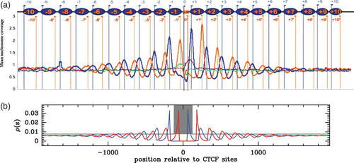
Figure 20. Statistical periodic ordering observed near an energy barrier as a fuction of the barrier height. (a) Density profiles obtained by solving the Percus equation (16) in a flat energy landscape with a finite energy barrier of width l=180 bp centered at s=0 (gray area) and a chemical potential value μ˜=4 kT. The profiles correspond to barrier heights ranging from 1 kT (black) to 20 kT (red). (b) NRL l* (dots) and wall density value ρ(s=±90)=ρ _w (curves) as a function of the barrier height, extracted from the density profiles (see (a)) at different values of the chemical potential: μ=−1 kT (black), μ=0 kT (red), μ=4 kT (green) and μ=10 kT (blue).

Figure 21. Theoretical probability of nucleosome occupancy at each point of a box of size L bordered by two infinite walls. (a) Box large enough to shelter five nucleosomes (green). (b) Larger box where the two dotted configurations are possible; the weighted average of the 5 and 6 nucleosome crystal-like profiles yields an irregular-looking average profile (red). (c) Larger box where six nucleosomes can be inserted without being tightly packed. (d) Probability of crystal configurations with a fixed number n of nucleosomes with respect to the box size L. Vertical colored lines correspond to the inter-barrier distances L used respectively in (a), (b) and (c). While only one configuration has clearly the highest probability for (a) and (c), two configurations are equally probable in (b), which justifies the superposition. The distances are expressed in nucleosome length units (hard core length l).

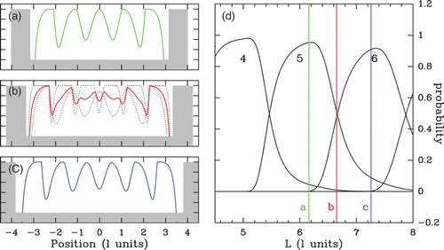
Figure 22. Theoretical NRL l* dependency on the box size L (see Figure 21); black dotted lines correspond to a fixed number n of nucleosomes and the red lines to the NRL size at a given chemical potential μ˜=4 kT. Vertical gray shaded bands correspond to the bistable domains. The distances are expressed in nucleosome length l units.

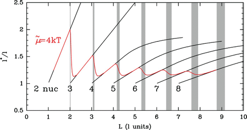
Figure 23. 2D-map of nucleosomes along budding yeast genes. (a) The 4554 genes are ordered vertically by the distance L between the first (5′) and last (3′) nucleosomes. The nucleosome occupancy profile of each gene is figured along a horizontal line: red dots correspond to the minima of nucleosome occupancy; nucleosomes occupy the white zones; in vivo data are retrieved from Lee et al. (2007). (b) Predictions of our theoretical modelling (blue) with fixed force boundary energy barriers (see text and Vaillant et al. (2010)) drawn on top of experimental data (red). Insets: mean experimental (red) and theoretical (blue) nucleosome occupancy profiles for crystal genes harboring 5 nucleosomes (right, top), 6 nucleosomes (right, bottom) and for bi-stable genes with 5/6 nucleosomes. (c) Zoom on the first 2000 genes in (b); gray-shaded areas correspond to some bi-stable L-domains. In (b) and (c), the black curves indicate the 5′ and 3′ end positions of the theoretical excluding nucleosome energy barriers.

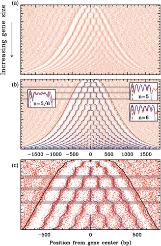
Figure 24. Our physical modelling consists of computing the energy cost to bend a DNA fragment of length l _w into almost two turns of the DNA double helix which are involved in the crystallized nucleosome particle (radius R=4.19 nm, pitch P=2.59 nm ). Adapted with permission from Richmond and Davey (2003). Copyright 2003 by Nature Publishing Group.

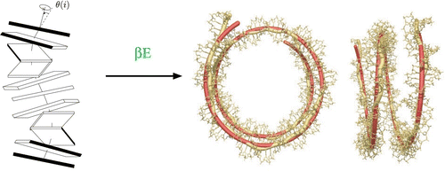
Figure 25. (a) 2D map representing the theoretical nucleosome occupancy probability P(s) [Equation (37)] along a 12 kbp long fragment of the budding yeast chromosome 2 as a function of the residual chemical potential (Chevereau et al. 2009): dark blue corresponds to low probability and red to high probability. The two white occupancy profiles are the theoretical profiles obtained for μ˜=−6 kT and−1.3 kT that correspond to a genome nucleosome coverage of 30% and 75% as observed in vitro (Kaplan et al. 2009) and in vivo (Lee et al. 2007) respectively; the corresponding in vitro and in vivo experimental nucleosome occupancy profiles are shown in red for comparison. (b) The corresponding energy landscape E(s) computed with the following parameter values: and l _w =125 bp (see text).

Figure 26. ln(ρ(s ₁)/ρ(s ₂)) versus Δ E ₁₂=E(s ₁)−E(s ₂), where ρ(s ₁) (resp. ρ(s ₂)) is the nucleosome density (computed as explained in the text, from the budding yeast genome) and E(s ₁) (resp. E(s ₂)) the nucleosome formation energy at the position s ₁ (resp. s ₂). The crosses correspond to two statistical samples in a diluted (μ˜=−6 kT, red) and dense (μ˜=0 kT, black) non-uniform fluid.

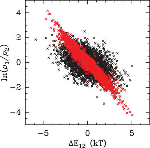
Figure 43. Energy landscape statistics (Δ E(s)=E(s)−Ē) computed with the following parameter values: δ=⟨(E−Ē)²⟩^1/2=2 kT and l _w =125 bp. The colors correspond to the LRC genomic DNA sequence (green) and to its randomly shuffled uncorrelated version (black). (a) Δ E(s) along a 50 kbp long fragment of budding yeast chromosome 2. (b) Energy pdfs computed for the 16 yeast chromosomes. (c) Energy auto-correlation function C(Δ s)/C(0) vs Δ s.

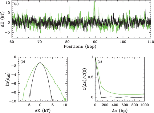
Figure 28. Comparison between the experimental occupancy profile from the in vitro MNase-seq experiment of Kaplan et al. (2009) (orange), the theoretical low-density occupancy profile (blue) and the energy landscape (green) (subsection “Intrinsic’ nucleosome formation energy landscape’) over regions of 10 kbp of several S. cerevisiae chromosomes. The theoretical predictions were obtained with the following parameter values: μ˜=−6 kT, δ=2 kT and l _w =125 bp.

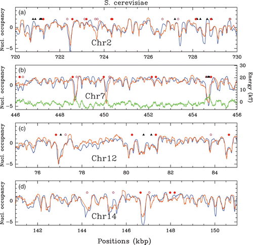
Figure 29. Histograms of Pearson correlation values r as measured in a 1 kbp sliding window between our physical modelling (μ˜=−6 kT, δ=2 kT and l _w =125 bp ) and the Kaplan et al. S. cerevisiae in vitro MNase-seq data (Kaplan et al. 2009) (light blue), Field et al. statistical model (Field et al. 2008) (pink) and a random occupancy landscape (black).

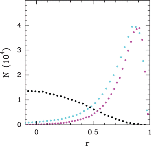
Figure 30. Comparing the predictions of our physical modelling (μ˜=−6 kT, δ=2 kT and l _w =125 bp ) with the Kaplan et al. S. cerevisiae in vitro MNase-seq data (Kaplan et al. 2009). (a) Histograms of nucleosome occupancy Y(s) values centered at their typical value: model (blue), in vitro data (orange). (b) Corresponding auto-correlation function C(Δ s)=⟨δ Y(s) δ Y(s+Δ s)⟩; the green curve corresponds to the auto-correlation function of the theoretical nucleosome formation energy profile (see the chromosome 7 panel in Figure 28).

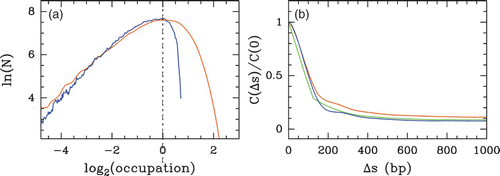
Figure 31. Comparison between the experimental occupancy profile from the in vivo MNase-chip experiment of Lee et al. (2007) (red), the theoretical high-density occupancy profile (blue) and the energy landscape (green) (subsection “Intrinsic’ nucleosome formation energy landscape’) over regions of 10 kbp of several S. cerevisiae chromosomes. The theoretical predictions were obtained with the following parameter values: μ˜=−1.3 kT, δ=2 kT and l _w =125 bp.

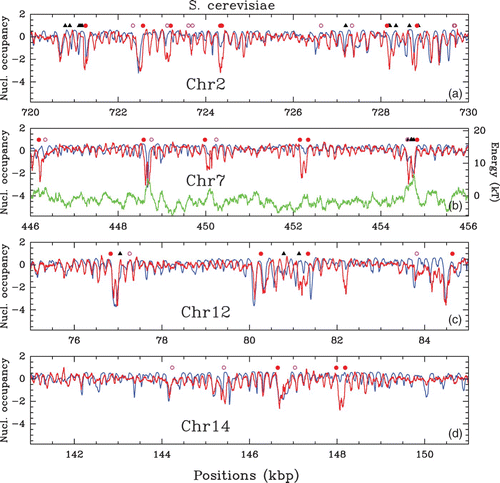
Figure 32. Histograms of Pearson correlation values r between the Lee et al. S. cerevisiae in vivo MNase-chip data (Lee et al. 2007) and our physical modelling (μ˜=−1.3 kT, δ=2 kT, l _w =125 bp ) (blue), Yuan and Liu (2008) model (pink) and a random occupancy landscape (black). The Pearson correlation was measured in a 1 kbp sliding window over the 16 yeast chromosomes: (a) no shift d=0 between the theoretical and experimental signal; (b) for a shift d _M that maximizes the correlation; (c) histogram of optimal shift d _M values. In (a,b), the green dots correspond to the histogram of Pearson correlation values obtained between the in vivo data and the theoretical nucleosome formation energy profile (actually with the affinity−E(s)) (see the chromosome 7 panel in Figure 31).

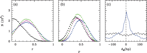
Figure 33. Comparing the predictions of our physical modelling (μ˜=−1.3 kT, δ=2 kT, l _w =125 bp ) with the Lee et al. (2007) S. cerevisiae in vivo MNase-chip data. (a) Histograms of nucleosome occupancy Y(s) values centered at their typical value: model (blue), in vivo data (red). (b) Corresponding auto-correlation function C(Δ s)=⟨δ Y(s) δ Y(s+Δ s)⟩.

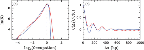
Figure 34. Histograms of local NRL: comparison of the predictions of our physical modelling (μ˜=−1.3 kT, δ=2 kT and l _w =125 bp ) for budding yeast (blue) (the same histogram is obtained for C. elegans) with the in vivo S. cerevisiae MNase-chip data of Lee et al. (2007) (red) and C. elegans MNase-seq data of Valouev et al. (2008) (green).

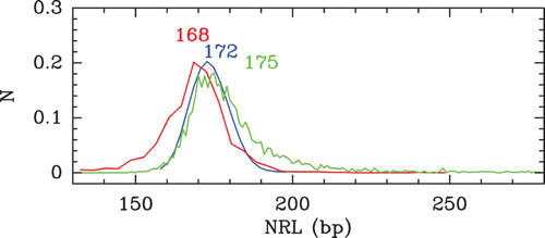
Figure 35. Nucleosome occupancy profiles observed in vivo (red) and predicted by our physical model for parameter values μ˜=−1.3 kT, δ=2 kT and l _w =125 bp (blue) along fragments of S. cerevisiae chromosome 2 (a), 7 (b), 2 (c) and 6 (d). For comparison also represented are the corresponding theoretical energy landscapes (green). The symbols represent the positions of TSS (red dots) and TFS (black triangle). The arrows at TSS indicate the transcription sense.

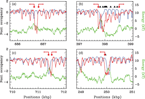
Figure 36. Comparison between our physical model predictions (μ˜=−1.3 kT, δ=2 kT, l _w =125 bp ) (blue) and in vivo nucleosome occupancy MNase-seq data (Tsankov et al. 2010, 2011) (orange): (a) S. kluyveri; 10 kbp fragment on chromosome C; (b) S. pombe; 10 kbp fragment on chromosome 2.

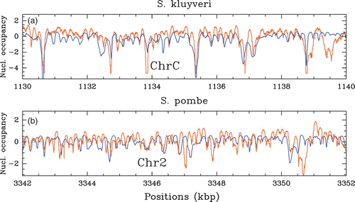
Figure 37. Comparison between our physical model predictions (μ˜=−1.3 kT, δ=2 kT, l _w =125 bp ) (blue) and the C. elegans in vivo nucleosome occupancy MNase-seq data (Valouev et al. 2008) (red): (a) and (b) correspond to two 15 kbp fragments of chromosome 1.

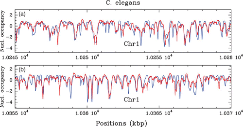
Figure 38. Histogram of Pearson correlation values r between our physical model (μ˜=−1.3 kT, δ=2 kT, l _w =125 bp ) and the Valouev et al. MNase-seq in vivo nucleosome occupancy data (Valouev et al. 2008) (see Figure 37). The Pearson correlation r was measured in a 10 kbp sliding window over the six C. elegans chromosomes.

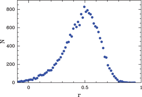
Figure 39. Comparison between our physical model predictions (μ˜=−1.3, δ=2 kT, l _w =125 bp ) (blue) and the in vivo nucleosome occupancy MNase-seq data obtained by Schones et al. (2008) in human CD4⁺ T cells (red). The four panels correspond to 10 kbp fragments of chromosome 6.

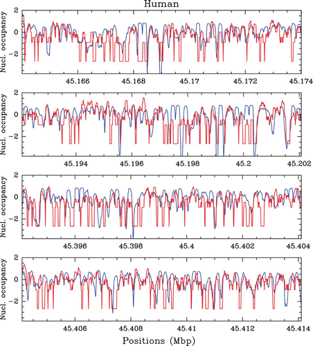
Figure 40. Performances of our physical model (μ˜=−1.3 kT, δ=2 kT, l _w =125 bp ) and of Yuan and Liu (2008) N-score model in terms of well-positioned nucleosomes as obtained by HMM methods. The comparison is made against the set of well-positioned nucleosomes obtained by Lee et al. (2007) on their S. cerevisiae in vivo experimental data using a similar HMM algorithm. Performance is measured by the proportion of true positive i.e. well-predicted positioned nucleosomes at a given overlapping distance of an experimental nucleosome. (a) Mean performance value versus the overlapping distance for the theoretical predictions of our physical model for the nucleosome occupancy profile (blue) and the energy landscape (green), and the Yuan and Liu N-score model (magenta). (b) Statistics of the performance values (at 35 bp accuracy) computed in a sliding window of size 5 kbp along the entire S. cerevisiae genome for our theoretical nucleosome occupancy predictions (blue) and for the random control (black). The vertical dashed lines (black and blue) indicate the corresponding mean values.

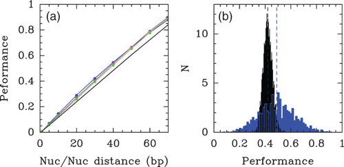
Figure 41. (a) Fraction in dinucleotides AA/TT/TA (3 bp moving average) at each position of centre aligned yeast, chicken and random chemically synthesized nucleosome-bound DNA sequences showing ∼10 bp periodicity of these dinucleotides. (b) Key dinucleotides inferred from the alignment are shown relative to the three-dimensional structure of one-half of the symmetric nucleosome. Adapted from Segal et al. (2006).

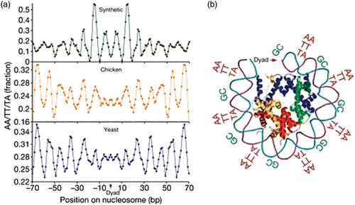
Figure 42. Power spectrum analysis of nucleosome occupancy profiles obtained from the in vivo data of Lee et al. (2007) (red), the in vitro data of Kaplan et al. (2009) (orange), the physical model described in the section ‘A sequence-dependent physical model of nucleosome occupancy’ for δ=2 kT and low μ˜=−6 kT (cyan) and high μ˜=−1.3 kT (dark blue) nucleosome density. For comparison, the green curve corresponds to the power spectrum of the formation energy landscape. The dashed lines correspond to the power-spectrum scaling exponent values ν=0.65, 0.74, 0.68, 0.74 and 0.46 from top to bottom corresponding to the following Hurst exponent values H=0.82, 0.87, 0.84, 0.87 and 0.77, respectively.

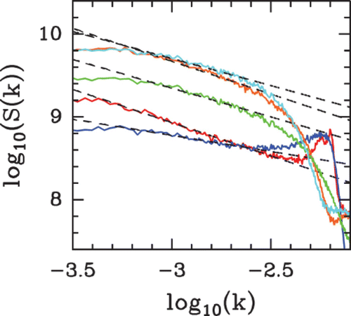
Figure 44. Comparison between the (G+C) content estimated in a 125 bp sliding window (black) and the S. cerevisiae in vitro nucleosome occupancy MNase-seq data of Kaplan et al. (2009) (orange). The horizontal line indicates the genome wide average (G+C) content value of 0.38.

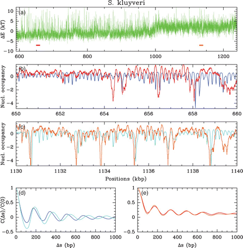
Figure 45. Comparison between the S. kluyveri in vivo nucleosome occupancy profile δ Y(s) of Tsankov et al. (2010) and the theoretical profile predicted by our physical model (see sections ‘Statistical positioning’ and ‘A sequence-dependent physical model of nucleosome occupancy’). (a) Formation energy landscape along the chromosome C computed with the following parameters δ=2 kT, l _w =125 bp; the high (G+C) content (52%) contig corresponds to the first 1 Mbp of the chromosome; low (G+C) content (G+C=40%) part corresponds to the last 250 kbp. (b,c) Comparison of the predictions of our physical modelling (μ˜=−1.3 kT ) (dark blue/cyan) with Tsankov et al. (2010) data (Figure 3) (red/orange) along a 10 kbp fragment of the high/low (G+C) content contig (indicated in (a) by the red/orange segments). (d,e) Corresponding auto-correlation functions C(Δ s)=⟨δ Y(s) δ Y(s+Δ s)⟩.

Lee , W , Tillo , D , Bray , N , Morse , R H , Davis , R W , Hughes , T R and Nislow , C . 2007 . A high-resolution atlas of nucleosome occupancy in yeast . Nat Genet. , 39 : 1235 – 1244 .

 Google Scholar

Schones , D E , Cui , K , Cuddapah , S , Roh , T- Y , Barski , A , Wang , Z , Wei , G and Zhao , K . 2008 . Dynamic regulation of nucleosome positioning in the human genome . Cell. , 132 : 887 – 898 .

 Google Scholar

Zhang , Z and Pugh , B F . 2011 . High-resolution genome-wide mapping of the primary structure of chromatin . Cell. , 144 : 175 – 186 .

 Google Scholar

Yuan , G- C , Liu , Y- J , Dion , M F , Slack , M D , Wu , L F , Altschuler , S J and Rando , O J . 2005 . Genome-scale identification of nucleosome positions in S. cerevisiae . Science. , 309 : 626 – 630 .

 Google Scholar

Whitehouse , I , Rando , O J , Delrow , J and Tsukiyama , T . 2007 . Chromatin remodelling at promoters suppresses antisense transcription . Nature. , 450 : 1031 – 1035 .

 Google Scholar

Kaplan , N , Moore , I K , Fondufe-Mittendorf , Y , Gossett , A J , Tillo , D , Field , Y , LeProust , E M , Hughes , T R , Lieb , J D , Widom , J and Segal , E . 2009 . The DNA-encoded nucleosome organization of a eukaryotic genome . Nature. , 458 : 362 – 366 .

 Google Scholar

Tsankov , A M , Thompson , D A , Socha , A , Regev , A and Rando , O J . 2010 . The role of nucleosome positioning in the evolution of gene regulation . PLoS Biol. , 8 : e1000414

 Google Scholar

Lantermann , A B , Straub , T , Strålfors , A , Yuan , G- C , Ekwall , K and Korber , P . 2010 . Schizosaccharomyces pombe genome-wide nucleosome mapping reveals positioning mechanisms distinct from those of Saccharomyces cerevisiae . Nat Struct Mol Biol. , 17 : 251 – 257 .

 Google Scholar

Tsankov , A , Yanagisawa , Y , Rhind , N , Regev , A and Rando , O J . 2011 . Evolutionary divergence of intrinsic and trans-regulated nucleosome positioning sequences reveals plastic rules for chromatin organization . Genome Res. , 21 : 1851 – 1862 .

 Google Scholar

Valouev , A , Ichikawa , J , Tonthat , T , Stuart , J , Ranade , S , Peckham , H , Zeng , K , Malek , J A , Costa , G , McKernan , K , Sidow , A , Fire , A and Johnson , S M . 2008 . A high-resolution, nucleosome position map of C. elegans reveals a lack of universal sequence-dictated positioning. . Genome Res. , 18 : 1051 – 1063 .

 Google Scholar

Shivaswamy , S , Bhinge , A , Zhao , Y , Jones , S , Hirst , M and Iyer , V R . 2008 . Dynamic remodeling of individual nucleosomes across a eukaryotic genome in response to transcriptional perturbation . PLoS Biol. , 6 : e65

 Google Scholar

Blank , T A and Becker , P B . 1995 . Electrostatic mechanism of nucleosome spacing . J Mol Biol. , 252 : 305 – 313 .

 Google Scholar

Tonks , L . 1936 . The complete equation of state of one, two and three-dimensional gases of hard elastic spheres . Phys Rev. , 50 : 955 – 963 .

 Google Scholar

Vaillant , C , Palmeira , L , Chevereau , G , Audit , B , d'Aubenton Carafa , Y , Thermes , C and Arneodo , A . 2010 . A novel strategy of transcription regulation by intragenic nucleosome ordering . Genome Res. , 20 : 59 – 67 .

 Google Scholar

Richmond , T J and Davey , C A . 2003 . The structure of DNA in the nucleosome core . Nature. , 423 : 145 – 150 .

 Google Scholar

Chevereau , G , Palmeira , L , Thermes , C , Arneodo , A and Vaillant , C . 2009 . Thermodynamics of intragenic nucleosome ordering . Phys Rev Lett. , 103 188103.

 Google Scholar

Yuan , G- C and Liu , J S . 2008 . Genomic sequence is highly predictive of local nucleosome depletion . PLoS Comput Biol. , 4 : e13

 Google Scholar

Segal , E , Fondufe-Mittendorf , Y , Chen , L , Thåström , A , Field , Y , Moore , I K , Wang , J-P Z and Widom , J . 2006 . A genomic code for nucleosome positioning . Nature. , 442 : 772 – 778 .

 Google Scholar