Figures & data
Table 1. Popular high-throughput NGS platforms, currently available in the market and the comparison between different characteristic features (sequencing chemistry, read lengths/throughput, run-time, template preparation and applications).
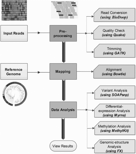
Figure 1. Steps for processing raw NGS data to generate the set of structural variants or genotype calls. Pre-processing steps include production of a set of reads in the form of NGS raw data. These reads undergo quality check, where separate quality score is assigned to each base read through base-calling algorithms, which often get recalibrated to measure the true error rates. In continuation, simple heuristic methods are applied to the individual data to improve overall quality scores of the reads. Depending upon the specific requirement, these processed data are further filtered, mapped and analyzed utilizing dozens of existing software packages and tools in the form of well pre-defined pipeline as shown in the figure.
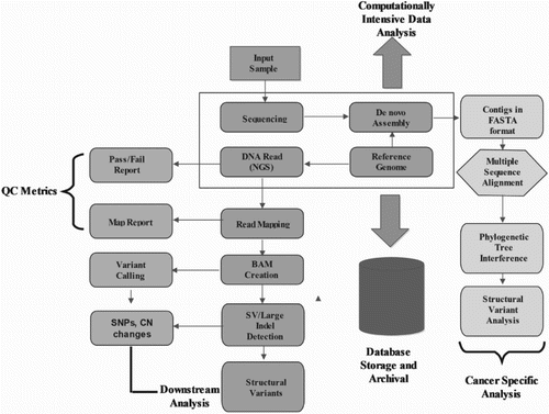
Figure 2. Data files are partitioned into large chunks and are replicated on multiple nodes.
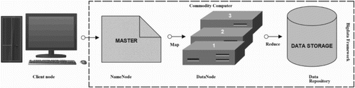
Figure 3. HDFS model is designed of two clusters, NameNode and DataNode, for processing large volume of data. These clusters are java-based applications, which run on a GNU/Linux operating systems only. Highly portable Java language facilitates nodes to run on various machines and this architecture affords high scalability in a number of deployed DataNodes. The complete functioning of the framework is explained in steps 1–6: Step 1 – MapReduce input files are loaded by Clients on the processing cluster of HDFS. Step 2 – The client posts job to processed files, the Mapper splits the file into key-value pairs and after the completion of the step, the involved nodes exchange the intermediate key-value pairs with other nodes. Step 3 – The split files are forwarded to Reducers (independent of knowledge of which Mapper it belongs to). Partitioners do this job more efficiently deciding the path of the intermediate key-value pairs. Step 4 – User-defined functions synthesize each key-value pair into a new object ‘Reduce-task’. Intermediate key-value pairs are sorted by Hadoop and then the job is shifted to Reducer. Step 5 – Reducer reduce() function receives key-value pairs, the value associated with the specific key are returned in an undefined order by the iterator. Step 6 – Results are regrouped and stored in outer files and governed by OutputFormat. The output files written by the Reducers are then left in HDFS for client’s use. Hence, the MapReduce application can introduce a high degree of parallelism and fault tolerance for the application running on it.
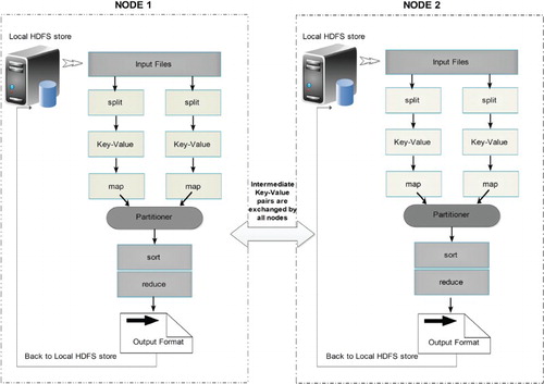
Figure 4. MapReduce data flow diagram illustrating the processing of complicated job and its components.
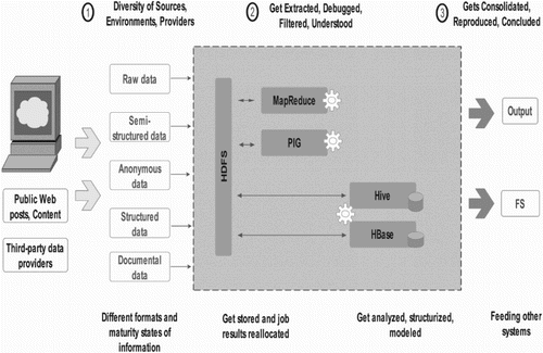
Figure 5. MapReduce, for short read mapping. Many subject reads are aligned with the reference using multiple compute nodes and detects variation. In this figure, nucleotide shown in the box depicts the variants.
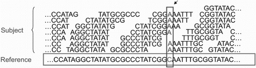
Table 2. Comparison of different features between packages – Crossbow, Seal, Eoulsan, FX, Distmap and Galaxy specifically used for distributed mapping.
Figure 6. A working pipeline of Crossbow used for whole genome resequencing combines Bowtie, for short read aligner, SoapSNP for identifying SNPs from high-coverage, short-read resequencing data. Hadoop allows Crossbow to distribute read alignment and SNP calling subtasks over a cluster of commodity computers.
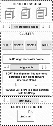
Figure 7. A working flowchart of NGS data analysis and the uses of various associated tools/pipelines.