Stabilization of piecewise-homogeneous Markovian switching CVNNs with mode-dependent delays and incomplete transition rates

Figures & data

Figure 1. Illustration of the piecewise-homogeneous evolution for systems with modes $r\left(t\right)\in \mathcal{S}=\{1,2\}$ and $\sigma \left(t\right)\in \mathcal{V}=\{1,2,3\}$.

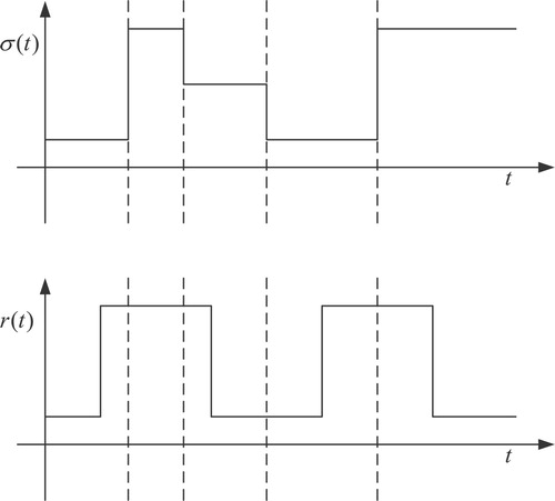
Figure 2. Variation of the homogeneous Markovian process $\sigma \left(t\right)$ with three modes.

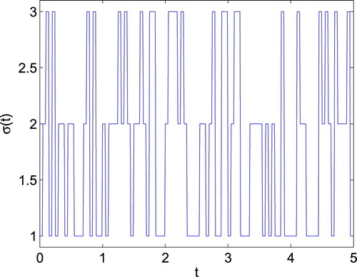
Figure 3. Variation of the piecewise-homogeneous Markovian process $r\left(t\right)$ with two modes.

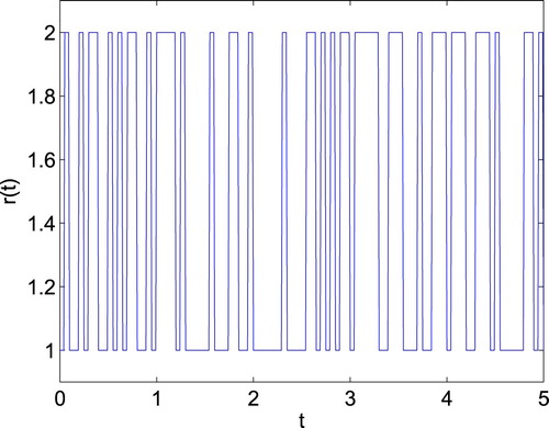
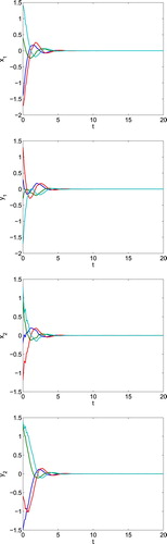
Figure 4. Time responses of the real/imaginary parts of state $z\left(t\right)$ for CVNN (1(1) $\begin{array}{rl}\dot{z}\left(t\right)& =-C\left(r\right(t\left)\right)z\left(t\right)+A\left(r\right(t\left)\right)f\left(z\right(t\left)\right)\\ & +B\left(r\right(t\left)\right)g\left(z\right(t-{\tau }_{r\left(t\right),\sigma \left(t\right)}\left(t\right)\left)\right)+\tilde{u}\left(t\right),t\ge 0\end{array}$(1) ) with $\tilde{u}\left(t\right)\equiv 0$ in Example 4.1.

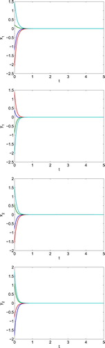
Figure 5. Time responses of the real/imaginary parts of state $z\left(t\right)$ for the open-loop system (1(1) $\begin{array}{rl}\dot{z}\left(t\right)& =-C\left(r\right(t\left)\right)z\left(t\right)+A\left(r\right(t\left)\right)f\left(z\right(t\left)\right)\\ & +B\left(r\right(t\left)\right)g\left(z\right(t-{\tau }_{r\left(t\right),\sigma \left(t\right)}\left(t\right)\left)\right)+\tilde{u}\left(t\right),t\ge 0\end{array}$(1) ) in Example 4.2.

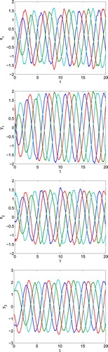
Figure 6. Time responses of the real/imaginary parts of state $z\left(t\right)$ for the closed-loop system (1(1) $\begin{array}{rl}\dot{z}\left(t\right)& =-C\left(r\right(t\left)\right)z\left(t\right)+A\left(r\right(t\left)\right)f\left(z\right(t\left)\right)\\ & +B\left(r\right(t\left)\right)g\left(z\right(t-{\tau }_{r\left(t\right),\sigma \left(t\right)}\left(t\right)\left)\right)+\tilde{u}\left(t\right),t\ge 0\end{array}$(1) ) in Example 4.2.