Deformation induced intermediate metastable lattice structures facilitate ordered B2 nucleation in a fcc-based high entropy alloy

Figures & data

Figure 1. TEM of the cold-rolled condition: (a) SADP pattern recorded along the [011]_fcc zone axis, and (b) the corresponding dark-field TEM (DFTEM) showing deformation twins. BSE of microstructures after annealing at 800°C for (c) 0.5 H (30 mins) and (d) 50H. The inset in (d) shows [011]_B2 micro-diffraction pattern.

Figure 2. Microstructural characterization after annealing at 800°C. (a) bright-field TEM (BFTEM) image showing B2 precipitation along twin-matrix interfaces. The inset shows the [011]_fcc SADP with the fcc-B2 Kurdjumov–Sachs (KS) orientation relationship. (b) A magnified BFTEM showing fcc-B2 interface. (c) HRTEM of the same fcc-B2 KS interface and the corresponding fast Fourier transform (FFT). In the FFT, [111]_B2 and [011]_fcc zone axes are indicated with a yellow hexagon and white rectangle, respectively. (d) STEM-EDS measurements comparing elemental concentrations in the fcc-matrix of the cold-rolled (Bulk-CR) condition prior to B2 precipitation, and elemental concentrations B2 in after 0.5 and 50H of annealing.

Figure 3. HRTEM of a twin along [011]_fcc in the cold-rolled condition. (a) Raw HRTEM image of a twin and the corresponding FFT as inset. (b) FFT of a HRTEM showing the twin-matrix interfacial region. The small arrow in the bottom left of panel ‘3b’ indicates distortion of the (002) plane by ∼11 deg. angle inside the twin. Here, the dotted white line shows the trace of distorted (002) plane and the bold white line is the (002) trace inside the twinned region far from the interface. Reference fcc lattices inside the (c) twin and (d) parent regions away from the twin-matrix interface is also shown.

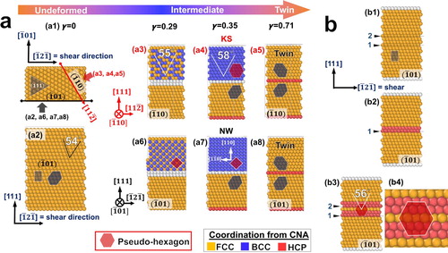
Figure 4. Two hard sphere models: (a) Borger–Burger–Olsen–Cohen model—(a1) and (a2) show two views of the undeformed fcc lattice, while (a3, a6), (a4, a7) and (a5, a8) show the same lattice after experiencing increasing shear strains. The top and bottom rows in panels (a3)–(a5) and (a6)–(a8) represent two views that are perpendicular to two conjugates {110}; as indicated in (a1), respectively. Note that panels (a3, a6) and (a4, a7) present the intermediate stages of shear where ‘bcc-like’ structures are observed, while (a5, a8) depicts the final stage corresponding to a twin. (b) Model showing local lattice deformation as due to stacking faults. Note that the CNA analysis of the shear structure also shows the resulting microstructure in three different colors, orange (fcc), blue (bcc) and red (hcp).