Hierarchical {332}<113> twinning in a metastable β Ti-alloy showing tolerance to strain localization

Figures & data

Figure 1. (a) Engineering strain-stress curve and true strain-stress curve of ST sample. The 2D full-field strain maps and the corresponding max of tensile strain (defined as ε_max) at different strain levels, as well as the bar of strain distribution, were also displayed in the inset of (a). The different strain levels were marked with the capital letter ‘A∼I’ in (a), respectively; (b) Strain-hardening rate vs true stress. The Considère’s criteria dσ/dε=σ line was also plotted in (b).

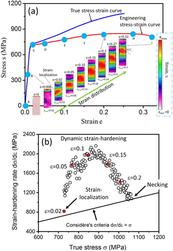
Figure 2. EBSD analysis of Ti-12Mo-10Zr sample at strain ε=0.1. (a) IPF map. The deformation bands were also symbolled by capital letters ‘A∼I’ with arrows, respectively; (b) Image quality (IQ) maps. The traces of slip bands were also marked with red arrows; and (c) Misorientation profile along the arrows labelled A and B in (a) as typical examples.

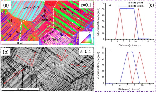
Figure 3. TEM images of the hierarchical structure of triple 332 T. (a) Bright-field image of triple 332 T (Lower magnification overview); (b) Close-up bright-field image of selected-area b in (a): matrix (M), primary 332 T, secondary 332 T and tertiary 332 T. The traces in the matrix and primary 332 T analysed by the trace method [14] were presented in (a). The selected-areas c, d, e and f were also highlighted by the dotted circle in (a) and (b); (c–f) SAED of selected-areas c, d, e and f, respectively. The zone axes (ZA) of the matrix is near [3$\overline{1}$5]_β, and the common ZA of [101]_β is shared by primary, secondary and tertiary 332 T.

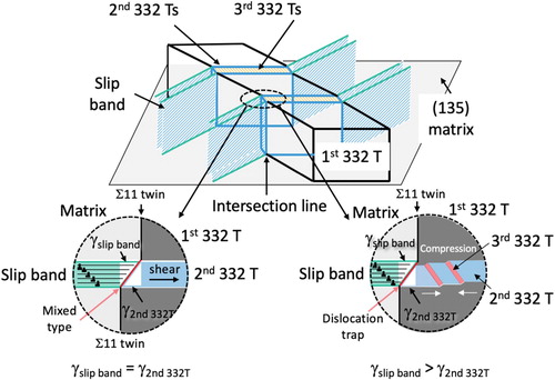
Figure 4. Schematic illustration of the 3D view and cross-sectional views concerning the formation sequence of primary 332 T, secondary 332 T and tertiary 332 T.

Marichal C, Van Swygenhoven H, Van Petegem S, et al. {110} Slip with {112} slip traces in bcc Tungsten. Sci Rep. 2013;3:2547. doi: 10.1038/srep02547

 PubMed Web of Science ®Google Scholar