Grain-subdivision-dominated microstructure evolution in shear bands at high rates

Figures & data

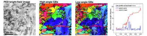
Figure 1. (a) SEM micrograph showing the morphology of micromarkers in a shear-banded chip of CP Ti cut with V₀ = 10 m/s. The black arrow indicates the shear displacement caused by shear banding. (b) Optical micrograph of shear bands in the chip.

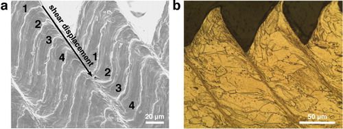
Figure 2. (a) Top-view EBSD IPF mapping of the machined strip. The shaded, narrow regions correspond to the shear bands. (b) A representative bright-field TEM micrograph covering a shear band and its neighborhood. The shear band boundaries are marked with dotted lines. (c) A bright-field TEM micrograph outside shear band and its corresponding SAED. (d) A magnified bright-field TEM micrograph in the center of a shear band and its corresponding SAED, showing the dramatically refined microstructure.

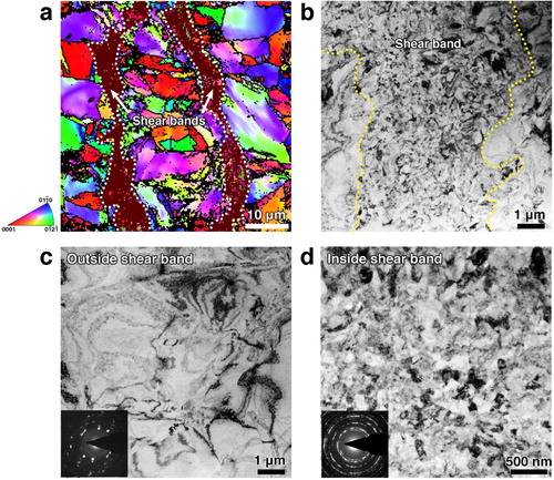
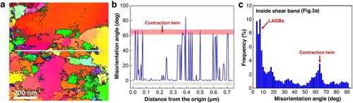
Figure 3. PED characterization of the microstructure in the center of shear band. (a) PED bright-field image. (b) HAGB (black) and (c) LAGB (gray) on top of the orientation map of the region of interest. The yellow dotted lines highlight a contraction twin. The numbered grains (1–4) in (a)–(c) are example of subgrains that are fully or partially bounded by LAGBs. (d) The misorientation line profile corresponds to the arrow in (c). (e) The correlative coefficient map of (a). (f) Zoomed-in view of the highlighted box in (d). The arrows indicate the presence of dislocations. (g) and (h) The PED patterns correspond to the labeled spots I and II in (e).

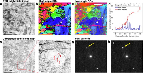
Figure 4. (a) A cropped PED map from Figure 3(b). (b) The misorientation line profile corresponding to the white arrow in (a). The shaded region highlights the contraction twin misorientation levels (65 ± 3°). (c) Misorientation angle distribution of inside-shear-band region in Fig.3a.