Introducing transformation twins in titanium alloys: an evolution of α-variants during additive manufacturing

Figures & data

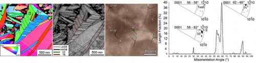
Figure 1. A typical microstructure in the Ti–6Al–4V alloy sample. (a) TKD phase map showing only the α’ phase. (b) TKD IPF map of three differently oriented variants clustered in a triangular shape. The three grains are marked with letters A, B, and C, respectively. A white arrow points to the central area of the clusters. (c) The corresponding GB map showing GB types, in which white, black, green, and red lines indicate low-angle GBs, high-angle GBs, V2 boundaries, and TBs, respectively. (d) and (e) $〈1\overline{2}10〉\text{and }\left\{10\overline{1}1\right\}$ pole figures from the areas marked with the green and blue squares in (c), respectively. The lower part of the $\left\{10\overline{1}1\right\}$ pole figures is further magnified and shown at the bottom of (d) and (e).

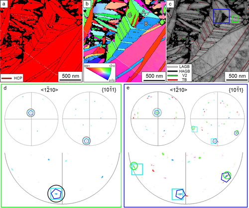
Figure 2. TEM analysis of a variant cluster area. (a) A STEM bright-field image taken from the same area as in Figure 1. Purple dashed lines and blue dashed lines mark primary and secondaries TBs, respectively. A black arrow points to the curved GBs between two clusters. (b) A corresponding SAED pattern generated from (a). Reciprocal lattices from the matrix, primary twins and secondary twins are marked with green, purple, and black dash lines, respectively. STEM-HAADF images taken from the orange, red, and blue square areas in (a) are shown in (c), (d) and (e), respectively. Red and green dashed lines marked TBs and V2 boundaries, respectively, in (c).

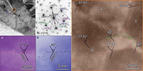
Figure 3. Microstructure in the water-quenched sample. (a) An EBSD IPF map showing three differently oriented variants clustered in a triangle shape. The three grains are marked as A, B, and C, respectively. (b) The corresponding GB map. White, black, green, and red lines mark LAGBs, HAGBs, V2 boundaries, and TBs, respectively. (c) and (d) The $1\overline{2}10$ and $\left\{10\overline{1}1\right\}$ pole figures, respectively, of grains A, B, and C revealing the three grains are separated by three 60°/$\left[1\overline{2}10\right]$ V2 inter-variant boundaries.

Figure 4. Misorientation profiles generated from EBSD data for (a) the water-quenched sample, and (b) the SLM sample.

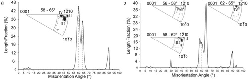
Table 1. Misorientation angle and rotation axis for each type of inter-variant boundaries and twinning systems in HCP Ti [14,28–30].

Structure	Rotation angle (°)	Rotation axis
V1	10.53	[0001]
V2	60	[$11\overline{2}0$]
V3	60.83	$\left[\overline{1.377}\overline{1}2.3770.359\right]$
V4	63.26	$\left[\overline{10}55\overline{3}\right]$
V5	90	$\left[1\overline{2.38}1.380\right]$
$\left(11\overline{2}1\right)11\overline{2}\overline{6}$ tensile twin	35.10	$10\overline{1}0$
$\left(11\overline{2}2\right)11\overline{2}\overline{3}$ compressive twin	64.62	$10\overline{1}0$
$\left(11\overline{2}4\right)22\overline{4}\overline{3}$ compressive twin	76.66	$10\overline{1}0$
$\left(10\overline{1}1\right)10\overline{1}\overline{2}$ compressive twin	57.42	$11\overline{2}0$
$\left(10\overline{1}2\right)10\overline{1}\overline{1}$ tensile twin	84.78	$11\overline{2}0$
$\left(11\overline{2}3\right)\overline{1}\overline{1}22$ tensile twin	86.98	$01\overline{1}0$

Beladi H, Chao Q, Rohrer GS. Variant selection and intervariant crystallographic planes distribution in martensite in a Ti-6Al-4V alloy. Acta Mater. 2014;80:478–489.

 Web of Science ®Google Scholar

Zhang X, Misra A. Superior thermal stability of coherent twin boundaries in nanotwinned metals. Scr Mater. 2012;66:860–865.

 Web of Science ®Google Scholar