Figures & data
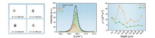
Figure 1. (a) Examples of depth-resolved diffraction patterns obtained at different X-ray energies from a volume 5–10 µm below the sample surface. (b) Radial X-ray line profile based on scans with different monochromatic energy. For calculating the radial profile, the diffracted intensity was summed in an interval of 0.030 nm−1 of the diffraction vector Q. The black circles are the calculated data from experimental diffraction patterns, while the black line is a fit to the calculated data by multiple Gaussian functions. The orange and olive lines are two subprofiles decomposed from the black line. The inset in (b) shows the fit result on a logarithmic scale.
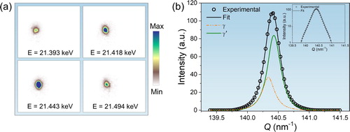
Figure 2. Quantitative results for the γ and γ′ phases at different depths determined based on the radial line profiles from tuning monochromatic energy. (a) FWHM of the radial profile δE. (b) Lattice constant a. (c) Lattice misfit Δγ/γ′ between two phases. (d) Apparent dislocation screening factor M*. (e) Apparent dislocation density ρ*. (f) The volume-weighted average apparent dislocation density ρ* over the two phases. The error bars in (a–c) are derived from profile separation using integrated intensity ratios of 25:75 and 35:65 between the γ and γ′ phases. Those of the dislocation densities (e–f) are based on the variations in FWHM in (a).
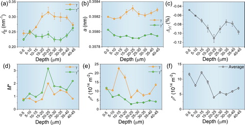
Figure 3. TEM image showing the dislocation structure of the Ni-based superalloy sample. In the upper part, γ and γ′ phases are labeled. A selected area electron diffraction pattern is inserted on the bottom right corner. Orange arrows mark a γ channel, where no dislocation is seen. The yellow arrow is parallel to the primary dendrite direction. The blue arrow indicates the direction of the microfocused X-ray beam.
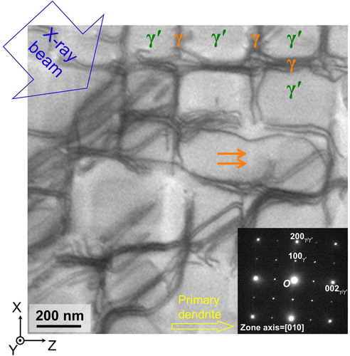
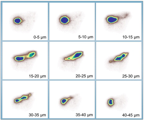
Figure 4. Pseudo white beam diffraction patterns, calculated by summing the diffraction patterns collected through a series of energies. From left to right and top to bottom, the depth is increased from 0–5 µm to 40–45 µm.