Figures & data
Figure 1. (a) Schematic illustration for the preparation of MP, MPI and MPIT, (b) SEM, (c) HRTEM, (d) TEM photo of MPIT, (e) EDX element mapping for MPIT.
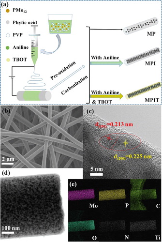
Figure 2. (a) XRD patterns, (b) Raman spectra. High-resolution XPS spectra, (c) Mo 3d, (d) P 2p, (e) N 1s. (f) Ti 2p of MPIT.
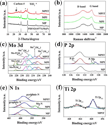
Figure 3. Sodium ion storage properties. (a) CV graphs of MPIT at 0.1 mV s−1; (b) initial three galvanostatic charging/discharging curves of MPIT at 100 mA g−1; (c) rate capability tests; (e) cycle performance at 1 A g−1; (d) initial 100 cycles; (f) EIS tests at open circuit voltage.
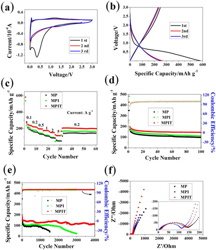
Figure 4. Electrochemical process kinetics analysis for MPIT. (a) CV curves at various sweeping rates from 0.1 to 0.9 mV s−1, (b) corresponding log i versus log v, (c) CV curve with pseudo-capacitance contribution shown by the shaded area at 0.5 mV s−1, (d) bar chart showing the capacitance percentage at different sweep rates, (e) EIS patterns collected after 100, 500, 1000 cycles and (e) corresponding relationship between Z’ and ω−1/2 for MPIT, the slope equals the Warburg coefficient (σw).
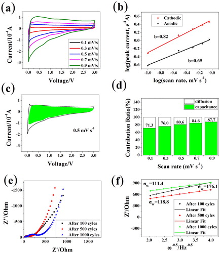
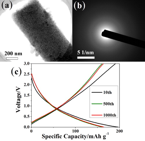
Figure 5. (a) TEM photos for expired electrode of MPIT, (b) SAED patterns and (c) representative charging-discharging curves at 1 A g−1.