Theory of cross phenomena and their coefficients beyond Onsager theorem

Figures & data

Figure 1. Fundamental components of materials science and engineering with (i) engineering focus and (ii) science focus [3].

Figure 2. Schematic diagram of energy landscape as a function of one internal process [1].

Figure 3. Relationships among tracer diffusivity, atomic mobility, kinetic L parameters, and intrinsic and chemical diffusivities.

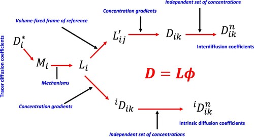
Figure 4. Calculated Seebeck coefficients for (i) PbTe for various p- and n-type doping levels [68]; (ii) p-type SnSe [68]; (iii) $L{a}_{2.75}T{e}_4$ [69].

Figure 5. Signs of the Soret coefficients in the water (H2O), ethanol (ETH), and triethylene glycol (TEG) ternary system at 25 C [96]. The colored regions denote regions of negative Soret coefficients of the respective components. Point Z marks the intersection of the boundaries of the three colored regions, where all three Soret coefficients vanish simultaneously. The steady state optical signal vanishes along the dashed line.

Figure 6. Simulated $C$ concentration profiles for 102 and 13,889 hours [87] with experimental data from ref [111] after 102 hours superimposed.

Figure 7. (i) Chemical potential of C in Fe-Si-0.45C alloys plotted with respect to the Si content at 1050°C with the TCFE9 thermodynamic database [113]; (ii) C composition profile in diffusion couple I after 13 days; (iii) C and Si compositions in the diffusion couple I with the numbers used to calculate the distance from the high Si side with the formula shown in the diagram.

Figure 8. Chemical potential of C in the Fe-0.80C alloy is increased only slightly by the Co content at 1000°C, calculated using a CALPHAD thermodynamic database and Thermo-Calc software [112,113].

Table 1. Physical quantities related to the first directives of molar quantities (first column) to potentials (first row), symmetric due to the Maxwell relations [1,11,345].

	T, Temperature	$\sigma$, Stress	$E$, Electrical field	$\mathcal{H}$, Magnetic field	${\mu }_i$, Chemical potential
S, Entropy	Heat capacity	Piezocaloric effect	Electrocaloric effect	Magnetocaloric effect	${\displaystyle \frac{\mathrm{\partial }S}{\mathrm{\partial }{\mu }_k}}$
$\epsilon$, Strain	Thermal expansion	Elastic compliance	Converse piezoelectricity	Piezomagnetic moduli	${\displaystyle \frac{\mathrm{\partial }{\epsilon }_{ij}}{\mathrm{\partial }{\mu }_k}}$
$\theta$, Electrical displacement	Pyroelectric coefficients	Piezoelectric moduli	Permittivity	Magnetoelectric coefficient	${\displaystyle \frac{\mathrm{\partial }{D}_i}{\mathrm{\partial }{\mu }_k}}$
$B$, Magnetic induction	Pyromagnetic coefficient	Piezomagnetic moduli	Magnetoelectric coefficient	Permeability	${\displaystyle \frac{\mathrm{\partial }{B}_i}{\mathrm{\partial }{\mu }_k}}$
$N_j$, Moles	Thermoreactivity	Stressoreactivity	Electroreactivity	Magnetoreactivity	${\displaystyle \frac{\mathrm{\partial }{N}_i}{\mathrm{\partial }{\mu }_k}}$, Thermodynamic factor

Table 2. Cross phenomenon coefficients represented by derivatives between potentials [23].

	$T$, Temperature	$\sigma$, Stress	$E$, Electrical field	$\mathcal{H}$, Magnetic field	${\mu }_i$, Chemical potential
$T$	$1$	$-{\displaystyle \frac{\mathrm{\partial }S}{\mathrm{\partial }\epsilon }}$	$-{\displaystyle \frac{\mathrm{\partial }S}{\mathrm{\partial }\theta }}$	$-{\displaystyle \frac{\mathrm{\partial }S}{\mathrm{\partial }B}}$	$-{\displaystyle \frac{\mathrm{\partial }S}{\mathrm{\partial }{c}_i}}$ Partial entropy
$\sigma$	${\displaystyle \frac{\mathrm{\partial }\sigma }{\mathrm{\partial }T}}$	$1$	$-{\displaystyle \frac{\mathrm{\partial }\epsilon }{\mathrm{\partial }\theta }}$	$-{\displaystyle \frac{\mathrm{\partial }\epsilon }{\mathrm{\partial }B}}$	$-{\displaystyle \frac{\mathrm{\partial }\epsilon }{\mathrm{\partial }{c}_i}}$ Partial strain
$E$	${\displaystyle \frac{\mathrm{\partial }E}{\mathrm{\partial }T}}$	${\displaystyle \frac{\mathrm{\partial }E}{\mathrm{\partial }\sigma }}$	$1$	$-{\displaystyle \frac{\mathrm{\partial }\theta }{\mathrm{\partial }B}}$	$-{\displaystyle \frac{\mathrm{\partial }\theta }{\mathrm{\partial }{c}_i}}$ Partial electrical displacement
$\mathcal{H}$	${\displaystyle \frac{\mathrm{\partial }\mathcal{H}}{\mathrm{\partial }T}}$	${\displaystyle \frac{\mathrm{\partial }\mathcal{H}}{\mathrm{\partial }\sigma }}$	${\displaystyle \frac{\mathrm{\partial }\mathcal{H}}{\mathrm{\partial }E}}$	$1$	$-{\displaystyle \frac{\mathrm{\partial }B}{\mathrm{\partial }{c}_i}}$ Partial magnetic induction
${\mu }_i$	${\displaystyle \frac{\mathrm{\partial }{\mu }_i}{\mathrm{\partial }T}}$ Thermodiffusion	${\displaystyle \frac{\mathrm{\partial }{\mu }_i}{\mathrm{\partial }\sigma }}$ Stressmigration	${\displaystyle \frac{\mathrm{\partial }{\mu }_i}{\mathrm{\partial }E}}$ Electromigration	${\displaystyle \frac{\mathrm{\partial }{\mu }_i}{\mathrm{\partial }\mathcal{H}}}$ Magnetomigration	${\displaystyle \frac{\mathrm{\partial }{\mu }_i}{\mathrm{\partial }{\mu }_j}}=-{\displaystyle \frac{\mathrm{\partial }{c}_j}{\mathrm{\partial }{c}_i}}={\displaystyle \frac{{\mathrm{\Phi }}_{ii}}{{\mathrm{\Phi }}_{ji}}}$ Crossdiffusion

Figure 9. Predicted phase diagrams of $Ce$ (i) temperature-pressure [245] with symbols for experimental data and (ii) temperature-volume [249] with purple diamond squares for thermal expansion anomaly and other symbols for experimental data.

Figure 10. Predicted phases diagrams of $F{e}_{3}Pt$ (i) temperature-pressure [250] with experimental data superimposed, noting pressure decrease from left to right, and (ii) temperature-volume [249] with experimental data (black circles) on the ambient pressure (0 GPa) volume curve and the purple diamonds for the anomalous regions of negative thermal expansions.

Figure 11. QCP phase diagrams: (i) temperature with respect to magnetic field of $YbR{h}_{2}S{i}_2$ with antiferromagnetic (AF), non-Fermi liquid (NFL), and Landau Fermi liquid (LFL) phase regions [213], (ii) temperature with respect to magnetic field of $YbR{h}_{2}S{i}_2$ and $YbR{h}_2(S{i}_{0.95}G{e}_{0.05}{)}_2$ with AF (blue left), NFL (yellow), and LFL (blue, right) phase regions [214], (iii) temperature with respect to pressure with contour map of electrical resistivity of Al-doped CrAs and pure CrAs [253], and (iv) temperature with respect to composition of $FeS{e}_{1-x}{S}_x$ with contour maps for electrical resistivity (ρ) and a parameter (A*) related to quasiparticle effective mass [255].

Figure 12. Superconducting phase diagrams, (i) cuprates [275], (ii) $Ce{M}_2{X}_2$ [256], (iii) $Ba(F{e}_{1-x}{M}_x{)}_{2}A{s}_2$ [276], and (iv) carbon- and hydrogen-doped $H_{3}S$ [277].

Figure 13. Orthorhombic-$BaF{e}_{2}A{s}_2$ (i) SDW ordering temperature ($T_{SDW}$, red curve) and characteristic temperature ($T_{\ast }$, blue curve) plotted with respect to pressure with experimental data (symbols) [282], and (ii) Fermi surface, Isosurfaces: (a) Stripe and (b) SDW; Cuts: (c) Stripe and (d) SDW; Top views of isosurfaces: (e) Stripe and (f) SDW [281].

Figure 14. Phase diagrams of (i) $T_C$ and normalized intensity of the superstructure spots as a function of pressure in Hg-1201 [303], (ii) $T$ plotted against hole concentration in Hg-1201 with hole concentration for (i) marked by the vertical rectangle and various phase regions [303], (iii) $T$ plotted against pressure in $FeS{e}_{1-x}{S}_x$ [304] with various phase regions: SDW (see Figure 13(i)), Tetra (tetragonal), Ortho (orthorhombic), M (magnetic), Nematic (no magnetic long-range), and SC (superconducting).

Figure 15. Gibbs energy diagram of an alloy system A-B with the effect of a driving force for diffusion acting over an interface between α and β, and the tangents describing the chemical potentials on both sides of the interface rotated relative to each other [326].

Figure 16. Dissolution of cementite at 910°C in an Fe-2.06Cr-3.91C (at. pct) alloy, (i) Isothermal section [120], (ii) Cr concentration profile after 1000 s [120], (iii) isothermal section with C activity plotted on the x-axis [334], (iv) transmission electron microscope (TEM) bright field image of cementite exhibiting Widmanstatten plates of α-bcc phase (γ-fcc at dissolution temperature) [334], and (v) TEM bright field image of extraction replica showing lamellar $M_7{C}_3$ structure ($u_{Cr}=0.54$ at point A) and untransformed $M{C}_3$ (darker area) [334].

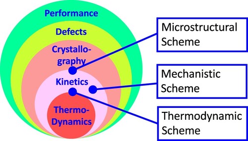
Figure 17. Classification schemes of kinetic processes in relation to fundamental components of materials science and engineering.

Liu ZK, Chen L-Q, Spear KE. An integrated education program on computational thermodynamics, kinetics, and materials design. https://www.tms.org/pubs/journals/JOM/0312/LiuII/LiuII-0312.html. 2003.

 Google Scholar

Liu Z-K. Computational thermodynamics and its applications. Acta Mater. 2020;200:745–792. DOI:https://doi.org/10.1016/j.actamat.2020.08.008.

 Web of Science ®Google Scholar

Wang Y, Hu Y-J, Bocklund B, et al. First-principles thermodynamic theory of Seebeck coefficients. Phys Rev B. 2018;98:224101. DOI:https://doi.org/10.1103/PhysRevB.98.224101.

 Web of Science ®Google Scholar

Wang Y, Chong X, Hu YJ, et al. An alternative approach to predict Seebeck coefficients: application to La 3−x Te 4. Scr Mater. 2019;169:87–91. DOI:https://doi.org/10.1016/j.scriptamat.2019.05.014.

 Web of Science ®Google Scholar

Schraml M, Bataller H, Bauer C, et al. The Soret coefficients of the ternary system water/ethanol/triethylene glycol and its corresponding binary mixtures. Eur Phys J E. 2021;44:128. DOI:https://doi.org/10.1140/epje/s10189-021-00134-6.

 PubMed Web of Science ®Google Scholar

Höglund L, Ågren J. Simulation of carbon diffusion in steel driven by a temperature gradient. J Phase Equilib Diffus. 2010;31:212–215. DOI:https://doi.org/10.1007/s11669-010-9673-0.

 Web of Science ®Google Scholar

Okafor ICI, Carlson ON, Martin DM. Mass transport of carbon in one and two phase iron-nickel alloys in a temperature gradient. Metall Trans A. 1982;13: 1713–1719. DOI:https://doi.org/10.1007/BF02647826.

 Web of Science ®Google Scholar

Thermo-Calc Databases. Available from: https://www.thermocalc.com/products-services/databases/.

 Google Scholar

Andersson JO, Helander T, Höglund L. THERMO-CALC & DICTRA, computational tools for materials science. CALPHAD. 2002;26:273–312. DOI:https://doi.org/10.1016/S0364-5916(02)00037-8.

 Web of Science ®Google Scholar

Liu ZK, Wang Y. Computational thermodynamics of materials. Cambridge: Cambridge University Press; 2016.

 Google Scholar

Liu Z-K. Ocean of data: integrating first-principles calculations and CALPHAD modeling with machine learning. J Phase Equilib Diffus. 2018;39:635–649. DOI:https://doi.org/10.1007/s11669-018-0654-z.

 Web of Science ®Google Scholar

Nye JF. Physical properties of crystals: their representation by tensors and matrices. Oxford: Clarendon Press; 1985.

 Google Scholar

Wang Y, Hector Jr LG, Zhang H, et al. A thermodynamic framework for a system with itinerant-electron magnetism. J Phys Condens Matter. 2009;21:326003. DOI:https://doi.org/10.1088/0953-8984/21/32/326003.

 Web of Science ®Google Scholar

Liu ZK, Wang Y, Shang S. Thermal expansion anomaly regulated by entropy. Sci Rep. 2014;4:7043. DOI:https://doi.org/10.1038/srep07043.

 PubMed Web of Science ®Google Scholar

Wang Y, Shang SL, Zhang H, et al. Thermodynamic fluctuations in magnetic states: Fe3Pt as a prototype. Philos Mag Lett. 2010;90:851–859. DOI:https://doi.org/10.1080/09500839.2010.508446.

 Web of Science ®Google Scholar

Gegenwart P, Custers J, Geibel C, et al. Magnetic-field induced quantum critical point in YbRh2Si2. Phys Rev Lett. 2002;89:056402. DOI:https://doi.org/10.1103/PhysRevLett.89.056402.

 PubMed Web of Science ®Google Scholar

Custers J, Gegenwart P, Wilhelm H, et al. The break-up of heavy electrons at a quantum critical point. Nature. 2003;424:524–527. DOI:https://doi.org/10.1038/nature01774.

 PubMed Web of Science ®Google Scholar

Park S, Shin S, Kim S-I, et al. Tunable quantum critical point and detached superconductivity in Al-doped CrAs. NPJ Quantum Mater. 2019;4:49. DOI:https://doi.org/10.1038/s41535-019-0188-6.

 Web of Science ®Google Scholar

Licciardello S, Maksimovic N, Ayres J, et al. Coexistence of orbital and quantum critical magnetoresistance in FeSe1-xSx. Phys Rev Res. 2019;1:023011. DOI:https://doi.org/10.1103/PhysRevResearch.1.023011.

 Google Scholar

Vittoria Mazziotti M, Jarlborg T, Bianconi A, et al. Room temperature superconductivity dome at a Fano resonance in superlattices of wires. Europhys Lett. 2021;134:17001. DOI:https://doi.org/10.1209/0295-5075/134/17001.

 Google Scholar

Monthoux P, Pines D, Lonzarich GG. Superconductivity without phonons. Nature. 2007;450:1177–1183. DOI:https://doi.org/10.1038/nature06480.

 PubMed Web of Science ®Google Scholar

Hosono H, Kuroki K. Iron-based superconductors: current status of materials and pairing mechanism. Phys C Supercond its Appl. 2015;514:399–422. Available from: https://linkinghub.elsevier.com/retrieve/pii/S0921453415000477.

 Web of Science ®Google Scholar

Snider E, Dasenbrock-Gammon N, McBride R, et al. Room-temperature superconductivity in a carbonaceous sulfur hydride. Nature. 2020;586:373–377. DOI:https://doi.org/10.1016/j.physc.2015.02.020.

 PubMed Web of Science ®Google Scholar

Wang Y, Shang SL, Chen LQ, et al. Magnetic excitation and thermodynamics of BaFe2As2. Int J Quantum Chem. 2011;111:3565–3570. DOI:https://doi.org/10.1002/qua.22865.

 Web of Science ®Google Scholar

Wang Y, Saal JE, Shang SL, et al. Effects of spin structures on Fermi surface topologies in BaFe2As2. Solid State Commun. 2011;151:272–275. DOI:https://doi.org/10.1016/j.ssc.2010.12.012.

 Web of Science ®Google Scholar

Izquierdo M, Freitas DC, Colson D, et al. Charge order and suppression of superconductivity in HgBa2CuO4+d at high pressures. Condens Matter. 2021;6:25. DOI:https://doi.org/10.3390/condmat6030025.

 Web of Science ®Google Scholar

Kreisel A, Hirschfeld P, Andersen B. On the remarkable superconductivity of FeSe and its close cousins. Symmetry (Basel). 2020;12:1402. DOI:https://doi.org/10.3390/sym12091402.

 Google Scholar

Ågren J. A simplified treatment of the transition from diffusion controlled to diffusion-less growth. Acta Metall. 1989;37:181–189. DOI:https://doi.org/10.1016/0001-6160(89)90277-0.

 Google Scholar

Liu Z-K, Höglund L, Jönsson B, et al. An experimental and theoretical study of cementite dissolution in an Fe-Cr-C alloy. Metall Trans A. 1991;22:1745–1752. DOI:https://doi.org/10.1007/BF02646498.

 Web of Science ®Google Scholar

Liu Z-K, Ågren J. Morphology of cementite decomposition in an fe-cr-c alloy. Metall Trans A. 1991;22:1753–1759. DOI:https://doi.org/10.1007/BF02646499.

 Web of Science ®Google Scholar