Harmonic structure, a promising microstructure design

Figures & data

Figure 1. A schematic illustration of relationships between true stress/strain diagram and work hardening rate curve from tensile test.

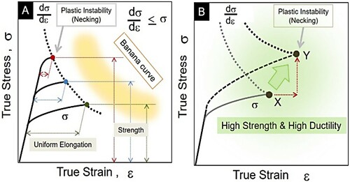
Figure 2. Schematic diagram of a harmonic structure material [10].

Figure 3. Three classifications of the harmonic structure. (a), (d): pure titanium, (b), (e): Ti64 alloy, (c), (f): SUS304L.

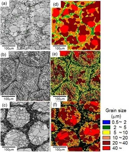
Figure 4. Tensile strength-elongation balance of SUS316L compacts.

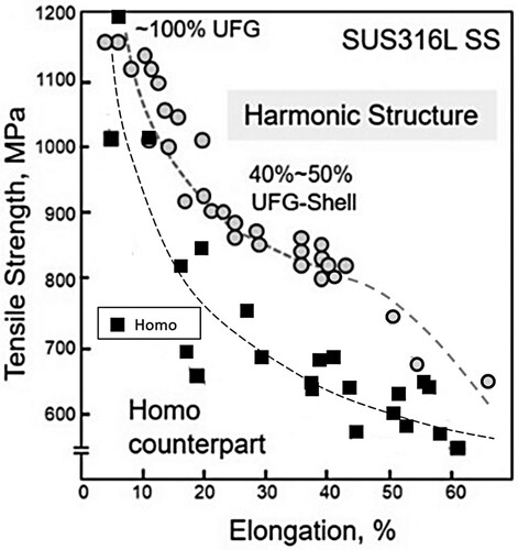
Figure 5. Mechanical properties of various harmonic microstructure materials.

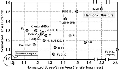
Figure 6. Microstructure and tensile test results of pure Ni HS and Homo compacts.

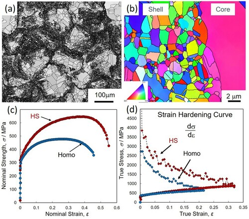
Figure 7. An EBSD and a TEM images showing the microstructure after tensile deformation of pure Ni harmonic material by 5%.

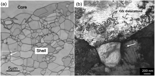
Figure 8. (a) An initial EBSD microstructure of a SUS304L HS sample. (b) The unloading-reloading curves. (c) Change of unloading yield stress σ_u, reloading yield stress σ_r, and back stress σ_b. Solid and open marks represent HS and Homo samples, respectively. (d) Variation of differences of the back stress with deformation between HS and Homo samples.

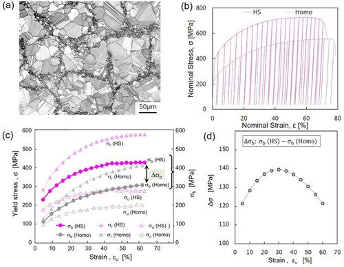
Figure 9. (a) EBSD images of the Homo, the HS, and the partial-HS materials, (b) tensile test results, and (c) the cross-sectional reduction rate.

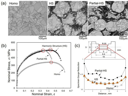
Figure 10. Experimental stress-strain curve for HS nickel shown alongside the results of analysis based on its fitting using the eq.(1) [28]. The latter reveals the evolution of stresses and strains in CG and UFG phases as well as the build-up of back stresses on the interface of core-shell regions.

Figure 11. Distribution of local equivalent strain (PEEQ) in the harmonic structure (HS) and heterogeneous (Hetero) materials with 40% UFG fraction at uniaxial tensile strain levels ε = 4% and ε = 10%. Note, at ε = 4% high-magnification areas are shown to illustrate local strain gradients, while at ε = 10% low-magnification areas are shown to cover the entire specimen cross-section with a global crack in Hetero.

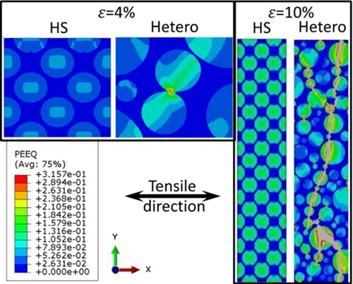
Figure 12. Schematic representation of the multiscale approach.

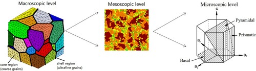
Figure 13. Harmonic microstructure mesh.

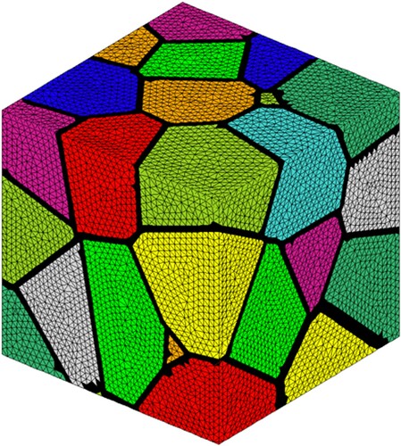
Figure 14. Simulation results and comparison experimental data.

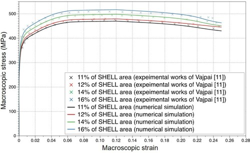
Figure 15. Comparison of simulated hysteresis loops and experimental data for HS CP-Ti.

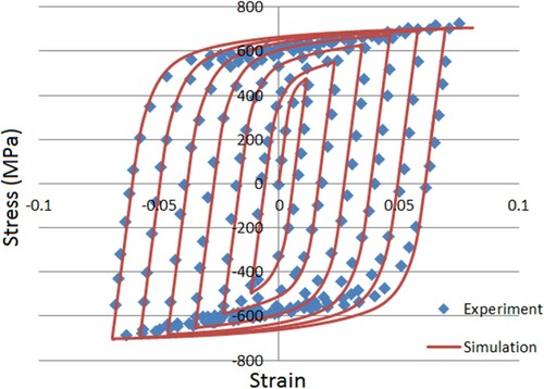
Figure 16. Distributionsc of (a) Effective shear strain fields and (b) effective strain fields in HS CP-Ti RVE.

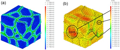
Figure 17. Schematic illustrating (a) Burgers orientation relationship in lamellar α + β colonies and (b) lamellar colony length scales.

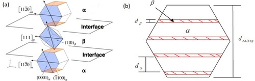
Figure 18. Distributions of (a) effective shear stress field and (b) effective shear strain field at the overall strain of 12.7% predicted by the simulation for HS Ti64.

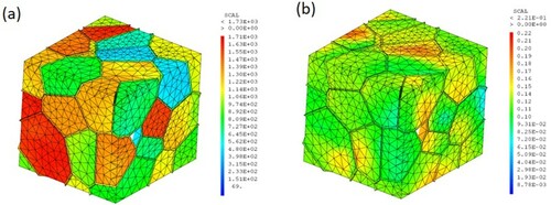
Figure 19. Stress-strain curves showing the strengthening of (a) pure Ti and (b) Ti64 caused by the HS design. The experimental and numerical data are plotted for comparison.

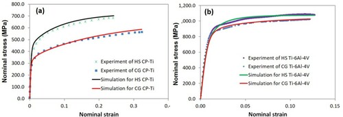
Figure 20. (a)–(c) are images extracted from an in-situ video sequence showing the operation of a source s in a prismatic plane. The source expands when a critical distance dc is reached. a-type dislocation exhibits screw segments with pinning points along their path (marked in (d), (e)) shows a pair of mixed dislocation in the basal plane, also highly pinned (f).

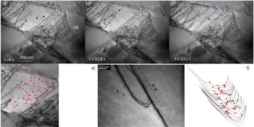
Figure 21. Overview of deformation at the shell-core interface between two holes in a TEM foil. In the core a marked shear band develops leading to a delocalized deformation in the shell. Inset: zoom in a shell grain showing numerous slip traces from the grain boundary (GB).

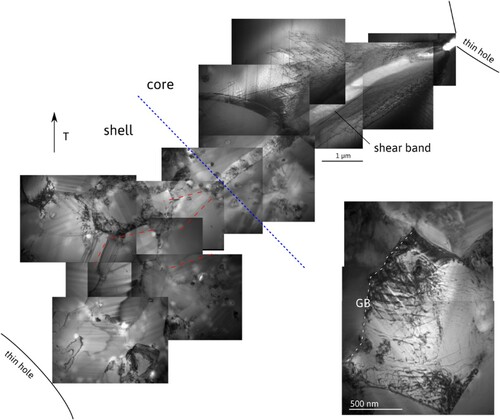
Figure 22. True stress versus true plastic deformation of the harmonic-structured (a) Ti and (b) Ti64 at R.T. (The strain rates in the dynamic regime for the different samples are shown in the inserts on figures (a) and (b), for Ti and Ti64). Evolution of the yield stress versus the strain rate of both Ti (‘Ti yield’) and Ti64 (‘Ti64 yield’) is shown in (c).

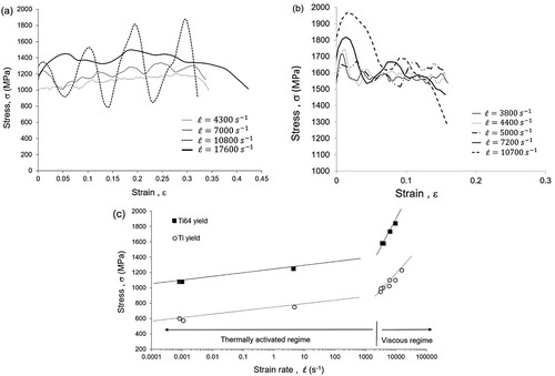
Figure 23. Microstructure of pure HS Ti. (a): IPF + Boundary map; (b) Homogeneous Ti after DHPB loading: IPF showing an ASB: (c) Zoom of (b); (d)–(f); DHPB loading on HS pure Ti under various conditions. Figures 23 (g)–(i) give the details on the formation mechanism of an ASB in pure Ti. (g): IPF map; (h) Grain boundary map: (i) Grain orientation spread (GOS) map. Figure 23 (h), in particular, reveals the presence of LAGBs, which means the UFG grains continue to bear a considerable amount of plastic deformation, as reported by [25]. (See text for details).

Figure 24. (a)–(d): Microstructural evolution in terms of GOS analysis. Apart from flattening the core-shell structure (Figs. b and d), the microstructure changes little qualitatively, whatever the dynamic strain rate. (The insert represents GOS values of the initial state). (e)–(g): HS Ti64 impacted at 3600 s⁻¹ and 50% compression strain. An ASB is seen, shearing the ultrafine-grained background microstructure formed through dynamic recrystallization. (e): SEM; (f) IPF; (g) Grain size map. (See text for details). (h-i): Heterogeneity of the deformation (view on the edge) on either side of an adiabatic shear band. Note the damage occurs within the shear band. 50% dynamic compression at a strain rate of 3800 s⁻¹. (See text for details)

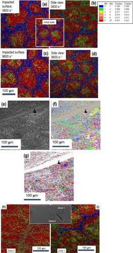
Figure 25. Results of four-point bending fatigue tests, showing stress amplitude as a function of cycles to failure explaining that HS series (Ti64) has the higher fatigue limit and fatigue life [21].

Figure 26. Plan views of the both fracture surfaces of the HS series (Ti64). (a) Fracture surface 1 (b) Fracture surface 2 [68].

Figure 27. SEM micrographs and IPF maps obtained by EBSD analysis for the facet observed in the fracture surfaces of the HS series (Ti64). (a) Fracture surface 1 (b) Fracture surface 2 [68].

Figure 28. IPF maps obtained by EBSD analysis for (a) HS and (b) TMP-HS series (CP titanium) near the crack initiation sites [63].

Figure 29. Relationship between da/dN and ΔK for the HS and untreated series (austenitic stainless steel) tested at R = 0.1 and 0.8 [71].

Figure 30. (a) SEM micrograph, (b) IPF map, and (c) grain size color map of a region near a crack profile (white lines) for the HS series (austenitic stainless steel) tested at R = 0.1 [71].

Figure 31. (a) SEM micrograph of the wear scar after fretting wear, and (b) schematic showing mechanism of wear, in the harmonic structure stainless steel.

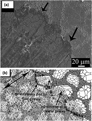
Figure 32. The schematic diagram shows the development of the Shell structure from the as-sintered state to successive thermo-mechanically processed (TMP) states.

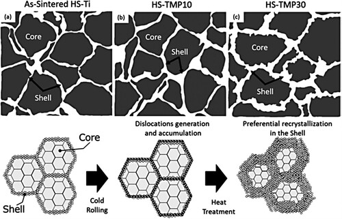
Figure 33. The nominal stress-strain curves of (a) Homo-Ti and (b) HS-Ti, respectively.

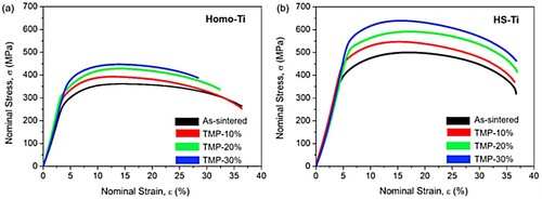
Figure 34. IPF and grain boundary map of structure of additively manufactured a heterogeneous Ti-Nb-Zr (Ta, Mo) high entropy alloy. (Courtesy Prof. G. Dirras).

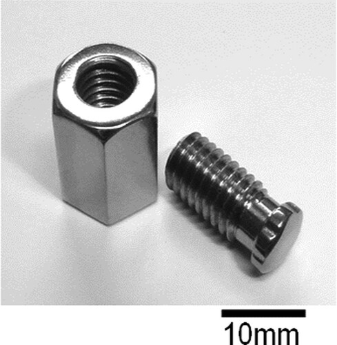
Figure 35. A set of pure Ti bolt and nut with the harmonic structure.

Sharma B, Dirras G, Ameyama K. Harmonic structure design: a strategy for outstanding mechanical properties in structural materials. Metals. 2020;10(12):1615.

 Web of Science ®Google Scholar

Orlov D, Kulagin R, Beygelzimer Y. Strain partitioning and back-stress evaluation in harmonic-structure materials. Mater Lett. 2020;275:128126.

 Web of Science ®Google Scholar

Dirras G, Ota M, Tingaud D, et al. Microstructure evolution during direct impact loading of commercial purity α-titanium with harmonic structure design. Matér Tech. 2015;103/311:1–9.

 Google Scholar

Kikuchi S, Kubozono H, Nukui Y, et al. Statistical fatigue properties and small fatigue crack propagation in bimodal harmonic structured Ti-6Al-4V alloy under four-point bending. Mater Sci Eng A. 2018;711:29–36.

 Web of Science ®Google Scholar

Kikuchi S, Hayami Y, Ishiguri T, et al. Effect of bimodal grain size distribution on fatigue properties of Ti-6Al-4V alloy with harmonic structure under four-point bending. Mater Sci Eng A. 2017;687:269–275.

 Web of Science ®Google Scholar

Osaki K, Kikuchi S, Nakai Y, et al. The effects of thermo-mechanical processing on fatigue crack propagation in commercially pure titanium with a harmonic structure. Mater Sci Eng A. 2020;773:138892.

 Web of Science ®Google Scholar

Kikuchi S, Nukui Y, Nakatsuka Y, et al. Effect of bimodal harmonic structure on fatigue properties of austenitic stainless steel under axial loading. Int J Fatigue. 2019;127:222–228.

 Web of Science ®Google Scholar