Dynamic mechanisms of strengthening and softening of coherent twin boundary via dislocation pile-up and cross-slip

Figures & data

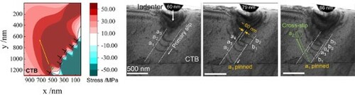
Figure 1. (a) EBSD map of the surface of the nickel cylinder used in indentation tests. The black frame marks the CTB selected for sample fabrication. (b) The setup of TEM-NanoIN test. The inset shows the SAED of the sample. (c) Crystallographic relationships in the experimental setup.

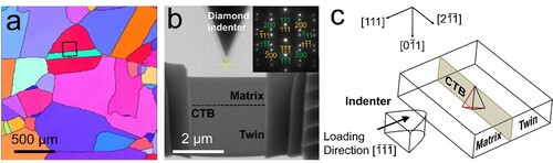
Figure 2. (a–e) Sequential TEM images showing abundant intra-grain cross-slip of dislocations piled up against a CTB. The labels at the top right corner of each image correspond to the indentation depth. (f) Dark-field TEM image of the area in the yellow frame in (e) viewed under $g=[\overline{2}11]$. (g) Stereographic projection and Thompson’s tetrahedron illustrating the crystallographic relationships of the primary slip and cross-slip planes. (h) TEM image of the sample after retraction of the indenter. The cross-slip traces are more evident, as shown by the green dashed arrows. (i) Schematic illustration of the origin of the multiple cross-slip events in (e).

Figure 3. (a) Schematic illustration of indentation in sample coordinates (C1). (b) Definition of stress tensors in a unit cell under indentation in C1 coordinates. (c) Schematic illustration of the relationship between the slip coordinate system (C2) and C1. (d and e) Stress fields created by a dislocation on primary and cross-slip systems in C1.

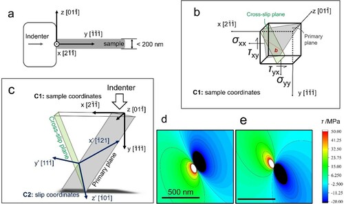
Figure 4. Analysis of the cross-slip of a₂. (a) TEM image taken just prior to the cross-slip of a₂. The slip planes and dislocations involved in cross-slip are denoted by solid lines and '⊥' signs, respectively. The CTB is marked as a red line. (b)–(e) Maps of stress distributions calculated for scenarios S1–S5 (in each map, a₂’s potential direction of motion is indicated by the green dashed arrow. The location of the cross-slip (CS) point in experiments is indicated by the green '⊥' symbol.): (b) Distribution of τ_p in Region I (marked by the black box in (a)); (c) Distribution of τ_c in Region II marked by the red box in (a); (d) Distribution of τ_c in Region I; (e) Distribution of τ_c in Region II (f) Comparison of the stress profiles in the vicinity of the CS point for each scenario.

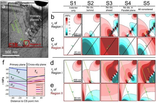
Table 1. Summary of scenarios considered in stress calculation.

Scenario	Contributors considered
S1	Indenter only
S2	Indenter + a1 (No dislocation behind)
S3	Indenter + a3, a4, b1, b2 and b3 (No dislocation ahead)
S4	Indenter + a1, a3 and a4 (No dislocation in parallel plane)
S5	Indenter + a1, a3, a4, b1, b2 and b3 (All considered)

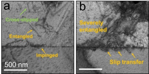
Figure 5. (a) Dislocation entanglement in the sample following further indentation. (b) Slip transfer after severe entanglement.