
Figures & data
Table 1. Comparison of solid solubility limits obtained by different non-equilibrium processing methods.
Table 2. Comparison of glass-forming composition ranges in different alloy systems processed by RSP and MA methods [Citation29].
Figure 1. XRD patterns of the blended elemental powder mixtures of (a) Fe42Al28Zr10B20 and (b) Fe42Co28Zr10B20 compositions as a function of milling time. An amorphous appeared on milling the Fe42Al28Zr10B20 powder mix for 20 h, and then a crystalline phase started to form from the amorphous matrix. The Fe42Co28Zr10B20 powder mix showed only a solid solution phase even after milling for 30 h. No amorphous phase formed in this powder blend.
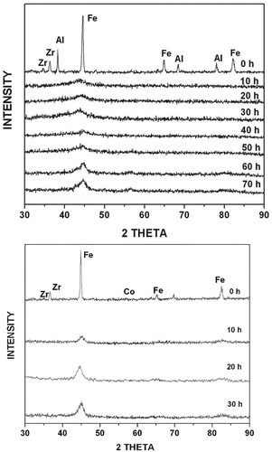
Table 3. Time required for glass formation in Fe42X28Zr10B20 alloys and the number of intermetallics in the respective binary phase diagrams.
Figure 2. XRD patterns of the blended elemental powder mixes milled for different times. (a) Fe42Ge28Zr10B20 powder mix mechanically alloyed for 10 and 60 h. While an amorphous phase formed on milling for 10 h, a crystalline phase (α-Fe) started appearing on continued milling up to 60 h. (b) Fe42Ni28Zr10C10B10 powder blend milled for 8 and 30 h. An amorphous phase appeared on milling the powder for 8 h, while the powder mix milled for 30 h showed the additional presence of some crystalline phases due to mechanical crystallization.
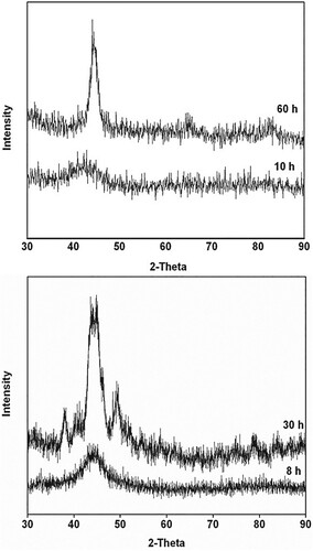
Figure 3. Hypothetical free energy versus composition diagram to explain the mechanism of mechanical crystallization in the Fe42X28Zr10B20 system. Note that point ‘‘1’’ represents the free energy of the blended elemental powders, point ‘‘2’’ formation of the α-Fe solid solution containing all the alloying elements in Fe, point ‘‘3’’ formation of the homogeneous amorphous phase, point ‘‘4’’ a mixture of the amorphous phase with a different solute content than at ‘‘3’’ and the α-Fe solid solution, and point ‘‘5’’ is for the equilibrium situation when the solid solution and intermetallic phases coexist.
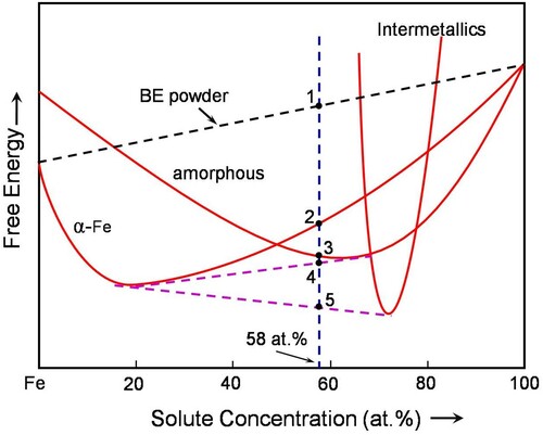
Figure 4. Variation of minimum grain size, dmin in mechanically milled FCC, HCP, and BCC metals as a function of the melting temperature of the metal. Note that even though the FCC and HCP metals show a decrease in grain size with increasing melting temperature of the metal, such a trend is not clearly seen in BCC metals. Further, when the melting temperature is very high (say >2000K), then the grain size remains almost unchanged irrespective of the melting temperature of the metal.
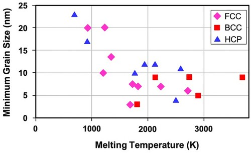
Figure 5. (a) Low-magnification and (b) high-magnification scanning electron micrographs of the γ-TiAl + 60 vol% ζ-Ti5Si3 composite specimen. The microstructure shows that the two phases are of ultrafine grain sizes, very uniformly distributed in the microstructure, and approximately of equal proportions. Such a microstructure is conducive to observing superplastic deformation under appropriate conditions of testing.
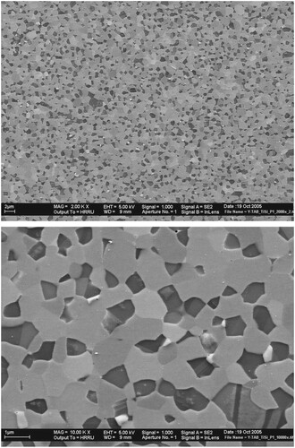
Figure 6. Tensile engineering stress vs. strain curves for the γ-TiAl + 60 vol% ζ-Ti5Si3 composite alloy tested at different temperatures and strain rates. The tests were conducted in air until fracture occurred.
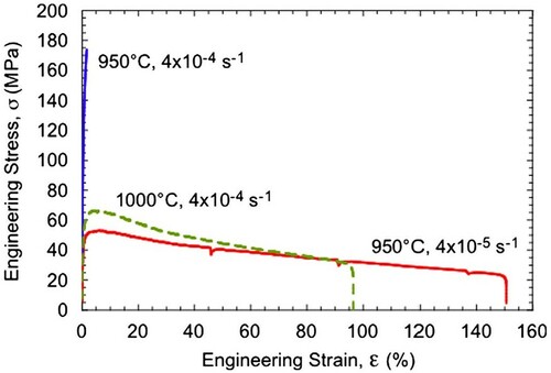
Figure 7. Transmission electron micrographs of the γ-TiAl + 60 vol% ζ-Ti5Si3 composite alloy (a) before and (b) after mechanical testing. Note that the grain size is still in the submicrometer range after testing and that there is dislocation accumulation in the γ-TiAl grains.
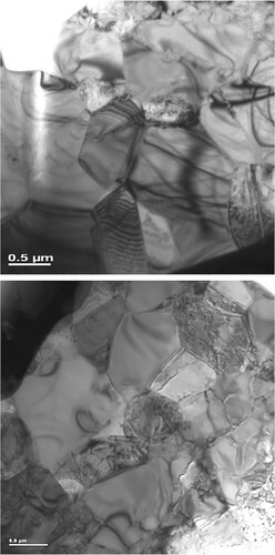
Figure 8. TEM microstructure of the hot-extruded composite from 30 h milled composite powders. (a) Bright-field TEM image. The yellow arrows indicate the presence of MGMC nanoparticles, and the blue arrows indicate the MgZn2 precipitates. (b) The interface between the α-Al matrix and the MGMC particle, which is clean and devoid of any undesirable products.
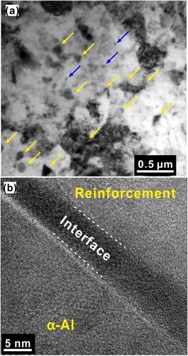
Figure 9. (a) The ultimate flow stress of the Al-7075 matrix and composites vs. volume fraction of the reinforcement at RT, 250°C, 350°C, 400°C, and 450°C. Note that while the strength increased with increasing volume fraction of the reinforcement at lower temperatures (RT and up to150°C), the strength decreased at higher temperatures. (b) Variation of the tensile yield strength of the Al-7075 matrix and composites as a function of the test temperature.
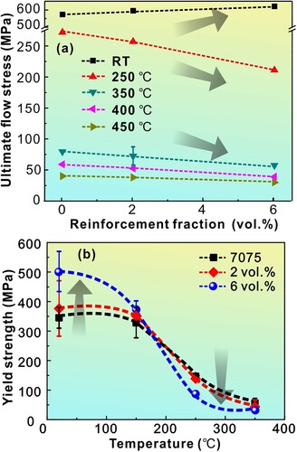
Figure 10. Electronegativity (Δχ) vs. atomic size difference (Δδ%) (Darken-Gurry plots) for the investigated HEAs. (a) for alloys processed by MA and (b) for alloys processed by all techniques. These plots clearly outline the Δχ vs. Δδ% regions for the different phases observed (FCC, BCC, amorphous, etc.).
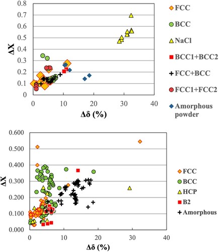
Table 4. Solid solubility extensions achieved in systems with a positive heat of mixing processed through MA.
Figure 11. Plot showing the relationship between heat of formation and the extended solid solubility limits achieved in alloy systems with a positive heat of mixing. It may be noted qualitatively that higher solid solubility limits have been achieved in alloy systems with a low positive heat of mixing and lower solubilities in systems with a high positive heat of mixing. That is these two parameters move in opposite directions.
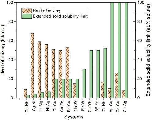
Figure 12. Typical heterostructures currently investigated. (a) Heterogeneous lamellar structure, (b) laminate structure, (c) gradient structure, and (d) harmonic (core-shell) structure. The smallest features in all these schematics are of nanometer dimensions, while the other features depend on the fabrication process [Citation155].
![Figure 12. Typical heterostructures currently investigated. (a) Heterogeneous lamellar structure, (b) laminate structure, (c) gradient structure, and (d) harmonic (core-shell) structure. The smallest features in all these schematics are of nanometer dimensions, while the other features depend on the fabrication process [Citation155].](/cms/asset/2cc39ede-f7b3-41b0-90d1-1f710ae900af/tmrl_a_2075243_f0012_oc.jpg)
Figure 13. Actual micrographs of some heterostructured materials. (a) EBSD image of initial coarse-grained equiaxed pure titanium [Citation153], (b) EBSD image of heterogeneous lamellar Ti after partial recrystallization [Citation153], and (c) shows a transmission electron micrograph of a copper specimen that exhibits bimodal distribution of grain sizes. This specimen was rolled at liquid nitrogen temperature to 93% cold work and then annealed at 200°C for 3 min. This latter treatment produced about 25 vol.% of grains with sufficiently large sizes [Citation151].
![Figure 13. Actual micrographs of some heterostructured materials. (a) EBSD image of initial coarse-grained equiaxed pure titanium [Citation153], (b) EBSD image of heterogeneous lamellar Ti after partial recrystallization [Citation153], and (c) shows a transmission electron micrograph of a copper specimen that exhibits bimodal distribution of grain sizes. This specimen was rolled at liquid nitrogen temperature to 93% cold work and then annealed at 200°C for 3 min. This latter treatment produced about 25 vol.% of grains with sufficiently large sizes [Citation151].](/cms/asset/009ffa9f-9160-48db-bc22-465920661d6f/tmrl_a_2075243_f0013_oc.jpg)