Figures & data

Figure 1. (a) Grain morphology (GM) of the samples: (I) H1; (II) H2; (III) H3; (IV) H4; (V) H5, (b) lines AB drawn in x–y planes, (c) magnification of the misorientation profile showing the different regions, (d) average major and minor width as hatch spacing changes, (e) misorientation angle profile along line AB.
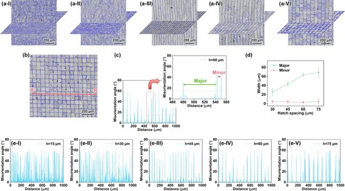
Figure 2. Inverse pole figure (IPF) maps of the samples (I) H1, (II) H3 and (III) H5 along the (a) x-, (b) y- and (c) z-directions in the x–y plane; (d) kernel average misorientation (KAM) map; (e) corresponding pole figures (PFs).
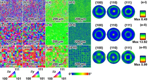
Figure 3. (a) Back-scatter electron (BSE) images of the samples: (I) H1; (II) H3; (III) H5; (b) IPF map along the BD and grain boundary (GB) distribution; (c) KAM maps.
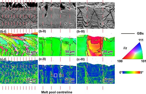
Figure 4. (a) Representative nanoindentation load-displacement curves; (b) ultrasonic attenuation and (c) average microhardness of the SCGs dominating samples; (d) microhardness map of the samples: (I) H2; (II) H3; (III) H4; (IV) H5.
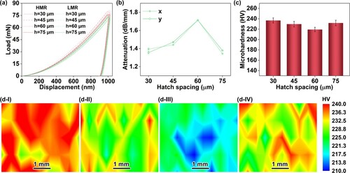
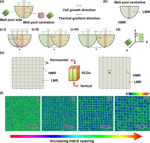
Figure 5. (a) Schematic illustration depicting solidification of the cell in single melt pool; (b) corresponding distinct regions (LMR and HMR) in single melt pool; (c) effect of the melt pool overlapping on the cell growth under small hatch spacing (I), large hatch spacing (II) and extra-large hatch spacing (III); (d) lattice rotation with 90° scan rotation strategy. (e) LMRs and HMRs in samples; (f) KAM maps of samples: (I) H2; (II) H3; (III) H4; (IV) H5.