Enhanced strength and ductility of metal composites with intragranularly dispersed reinforcements by additive manufacturing

Figures & data

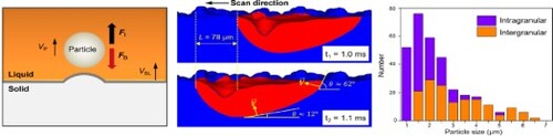
Figure 1. Theoretical analysis of particle engulfment in metal composites by SLM. (a) Schematic of particle motion. F_I and F_D stand for repulsive and drag force, respectively. V_SL and V_P are velocities of solidification front and particle motion, respectively. Gravity and buoyancy are not shown due to their small values. (b) The plot of net force as a function of V_SL. V_c is critical pushing velocity. (c) The dependence of V_c on particle radius (R). The size ranges of TiB₂ particles used in this work are shown. (d) Modeling results on V_SL calculation. V_SL = V sinθ. V is scanning speed (L/Δt). SD means scan direction. (e) The simulated 3D-temperature gradient profile. X, Y and Z are scan direction, transverse direction and sample building direction, respectively. Inset shows a schematic of melt flow during SLM.

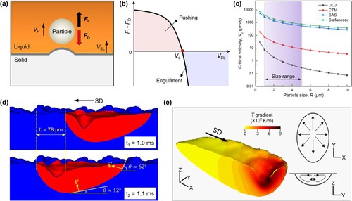
Figure 2. Microstructures of as-built TiB₂-Al composites. Both SLM and PM TiB₂-Al composites possess relative density of larger than 99.5%. (a) EBSD image showing the distribution of TiB₂ particles (colored in green, 15 vol.%) in SLM composite. High-angle grain boundaries (HAGBs) with misorientation larger than 10° are superimposed. (b) EBSD image of comparing PM TiB₂ (15 vol.%)-Al composite. The non-identified regions are shown in black. (c) EBSD image of PM composite after cold rolling. (d) Histogram showing the size distribution of TiB₂ particles and their locations either in grain interiors or at GBs, as measured by EBSD. (e) A typical APT slice (thickness 10 nm) showing the atomic distributions across the TiB₂-Al interface. The right panel shows the corresponding 1D compositional profiles.

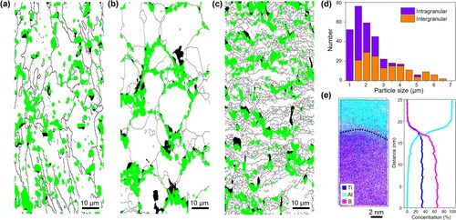
Figure 3. Crystallographic relationship between TiB₂ and Al in SLM TiB₂-Al composite. (a) and (b) are inverse pole figures showing the orientation of Al matrix parallel to the [0001] direction of the intragranularly and intergranularly distributed TiB₂ particles, respectively.

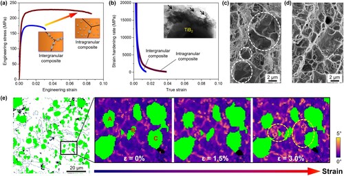
Figure 4. Mechanical properties and deformation mechanisms. (a) The representative tensile stress–strain curves of SLM composite and PM TiB₂-Al composite. (b) The plots of strain hardening rate as a function of true strain. Note that the strain hardening rate data after necking (which corresponds to true strain values of 1.4% and 3.9% for PM and SLM TiB₂-Al composite, respectively) are not shown due to the non-uniform deformation. Inset shows the representative TEM image of the deformed SLM composite. Numerous dislocations, as indicated by black arrows, are present at the interface. (c) and (d) are fracture surfaces of PM and SLM composite, respectively. TiB₂ are found at the fracture surface of PM sample, as indicated by the white dashed circles. (e) Ex-situ EBSD measurements for SLM composite with different strains (tensile strain: 0%, 1.5% and 3.0%). A, B and C are typical TiB₂ particles that are distributed inside Al grains. They are selected for further EBSD examinations. KAM maps, measured in degrees, are used to illustrate the heterogeneous deformation inside Al grains. Local misorientations (or GNDs) show obvious increments with strain nearby the intragranular TiB₂ particles, as indicated by the yellow dashed circles.