Figures & data

Figure 1. Schematic diagram of a single track. The cross-section A-A is parallel to the scan direction and perpendicular to the substrate. The cross-section B-B is perpendicular to the scan direction and the substrate. The melt pool depth (Dm) is the distance from the melt pool bottom to the substrate top. The melt pool width (Wm) is the track width on the substrate top.
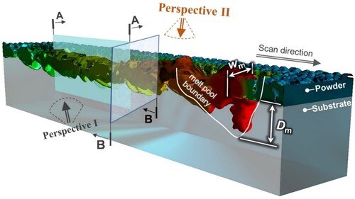
Figure 2. Alloy composition distributions obtained from single-track experiments (a) and simulations (b) on cross-sections A-A with L = 100 W and V = 300 mm/s. Fe and Ni are the principal elements in 316L (Fe 65.5%, Ni 12.5%) and IN718 (Fe 16.9%, Ni 52.5%) respectively. For the clarity purpose, we refer to Fe (in red brown) rich area as the representation of 316L, and Ni (green) rich area as the representation of IN718. The 2D component gradient distribution (c) and their corresponding 3D component gradient isosurface shape (d) of 316L/IN718 is obtained from our numerical simulations. Figure (d) is viewed from viewing angle I in Figure . In Figures (a) and (b), the positions of points A, B and C, indicated by the arrows, are used for extracting the Ni element content.
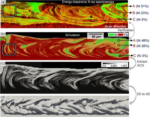
Figure 3. Composition distribution, composition gradient and microstructure of dissimilar alloys obtained using EDS and EBSD under L = 200 W and V = 1500 mm/s, see (a). Composition distribution, composition gradient and microstructure under L = 100 W and V = 300 mm/s, see (b). Schematic diagram of curved grain angle, see (c). Curved grain shape characteristics under different process parameters, see (d). Figures (a) and (d) are extracted from the cross-section B-B. Figure (b) is extracted from the cross-section A-A. In Figure (b), EDS images are displayed in black and white, where the white and black areas represent 316L and IN718, respectively. A data extraction line is selected in the EDS image, and the positions of pure 316L and pure IN718 are represented by reddish-brown and green colors, respectively.
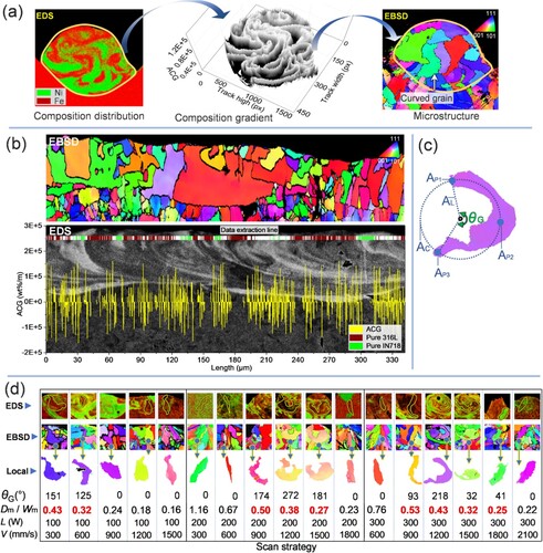
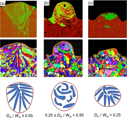
Figure 4. Schematic illustration of the mechanism by which temperature gradient (a), composition gradient (b) and mixed (c) modes dominate the growth of curved grains, respectively. (a) is 200 W and 300 mm/s, (b) is 300 W and 1200 mm/s and (c) is 200 W and 1800 mm/s.