Figures & data
Figure 1. Illustration of both an object and fluid within a computational cell as described by the improved FAVOR method used in this study.
Figure 2. Interface region between the 2D NSWE and 3D RANS model in 2CLOWNS-3D with the necessary variables required for coupling shown. The subscripts have the following definitions: is the x-direction flux (defined on cell edge),
is the y-direction flux (defined on cell edge),
is the center cell (free surface) or edge (velocities) between model interface,
is the one cell/edge west of center,
is the one cell/edge east of center,
is the two cells/edges east of center,
is the one cell/edge north of center,
is the one cell/edge south of center,
is the left half of the sub-grid,
is the right half of the sub-grid,
is the upper half of the sub-grid, and
is the lower half of the sub-grid.
Figure 3. (a) Bathymetry in the largest 2DH NSWE mesh layer (resolution is 1350 m) with dashed black rectangles indicating the boundaries of the four other higher resolution 2DH NSWE mesh layers (450, 150, 50, 10 m). The red–blue filled contour plot shows the total vertical deformation of the ground due predicted by the Satake v8.0 (Satake et al., Citation2013) source model of the 2011 Tohoku-oki Earthquake Tsunami (note that absolute vertical deformation smaller than 0.2 m is not plotted for figure clarity purposes). Annotated triangles indicate the locations of the four offshore GPS buoys closest to Kamaishi Bay. (b) Bathymetry/Topography up to T.P. +40 m in the highest resolution 2DH NSWE mesh layer (10 m) with the offshore tsunami breakwater included. The dashed black rectangle indicates the boundary of the 3D RANS mesh.
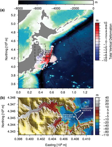
Figure 4. Sketch of Kamaishi Bay breakwater with the damaged caissons shaded red and yellow. Front on view and cross-section of the submerged breakwater opening; adapted from Arikawa et al. (Citation2012).
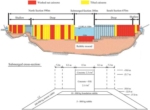
Figure 5. Time series of surface elevation (T.P. m) at the four GPS buoys operated by PARIa2011 that are closest to Kamaishi Bay during the 2011 Tohoku-oki Earthquake Tsunami. Comparison of 2CLOWNS-3D simulation results using the Satake v8.0 kinematic source model (Satake et al., Citation2013) with observations.
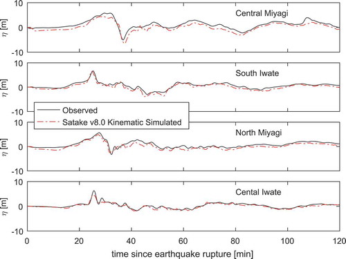
Figure 6. Filled contour plot of the maximum calculated free surfaces, ηmax (in T.P. m) from the 2CLOWNS-3D simulation on the 2DH NSWE 10 m mesh. Filled circles indicate TTJS survey measurements (Mori and Takahashi, Citation2012). The dashed rectangle indicates the location of 3D RANS mesh.
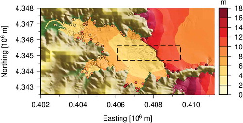
Figure 7. Comparison of run-up/inundation heights, ηmax from the 2CLOWNS-3D and 2DH NSWE model simulations versus TTJS survey measurements (Mori and Takahashi, Citation2012). Left plot shows the comparison in bays surrounding Kamaishi (Toni, Ryoishi, and Otsuchi), while the right plot shows the comparison inside Kamaishi Bay. The geometric mean and the geometric standard deviation
(Aida, Citation1978) between simulated and measured ηmax are also indicated.
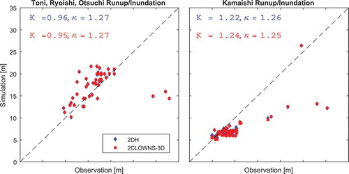
Figure 8. Time series of the horizontal volume flux per unit width (averaged in the north–south direction) over the submerged opening of the large-scale offshore breakwater during the 2DH NSWE and 2CLOWNS-3D simulations. Two 2DH NSWE simulations are conducted where;
= 0 and,
= 0.5.
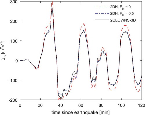
Figure 9. Time series of the forces on the submerged caissons for the 2CLOWNS-3D and 2DH NSWE simulations. (a) Magnitude of drag force per unit width, , (b) magnitude of overturning moment per unit width about the caisson heel,
. The shaded areas indicate the range of forces over the width of the submerged breakwater opening while lines indicate the mean value.
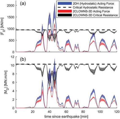
Figure 10. Filled contour plot of the maximum calculated magnitudes of the depth-averaged velocities, during model simulations on the 10 m 2DH NSWE mesh. (a) 2DH NSWE, (b) 2CLOWNS-3D dashed black rectangle indicates the extent of the 3D RANS domain.
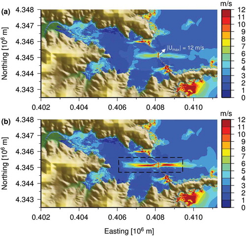
Figure 11. Comparisons of the maximum dimensionless bed shear stress, , around the breakwater opening assuming a uniform grain size,
mm, on the seabed and
cm over the rubble mound. (a) 2DH NSWE simulation, (b) 2CLOWNS-3D simulation using depth-averaged velocity, (c) 2CLOWNS-3D simulation using near-bed velocity. The main breakwater sections are plotted in gray.
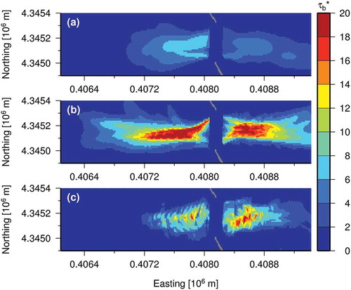
Figure 12. Velocity field vectors and dynamic pressure (difference from hydrostatic) colormap along the y = 4345,175 m northing cross-section inside the 3D RANS domain at t = 31.6 min (peak inundating flow) and t = 40.5 min (peak drawback) after the earthquake rupture. The left-hand side plots the entire 3D RANS model domain while the right-hand side zooms in closer to the breakwater.
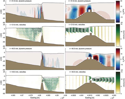
Figure 13. Schematic of the canonical wall jet under the current setting of flow through the submerged breakwater opening. The three regions of decay of the maximum (centerline) longitudinal velocity, , are indicated along with the approximate distances from the submerged breakwater opening that the regions extend to (based on a slenderness ratio
).
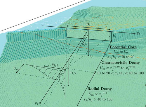
Figure 14. Time series of maximum (centerline) longitudinal velocities, at various longitudinal positions downstream from the submerged breakwater opening for the realizable
model simulation. The dashed black lines are the time series at
and
, and the solid blacks lines are those in the range
. Time averaging for analysis of jet characteristics is performed over the time interval where
is in the upper 20th percentile (indicated by the red lines) for the plotted interval at each longitudinal position.
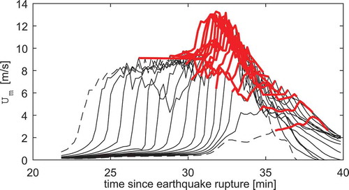
Figure 15. (a) Decay of the maximum (centerline) longitudinal velocity, , of the transient wall-jet with distance downstream of the breakwater; (b) growth of the half-width of the transient wall-jet in the horizontal,
,
, and vertical
planes. Left plots: Standard
model; Right plots: realizable
model; Regions I: potential core; II: characteristic decay; III: radial decay.
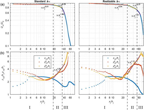
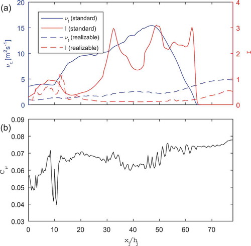
Figure 16. (a) Maximum values of the turbulent viscosity, , and turbulent intensity,
, along the centerline of the transient wall-jet with distance downstream of the breakwater comparing the standard and realizable
models; (b) minimum values of the coefficient of turbulent viscosity,
, along the centerline with distance downstream of the breakwater for the realizable
model.