Figures & data
Figure 1. Fukude-Asaba Coast located 10 km west of the Tenryu River mouth. Sediments are transported from west to east. Waves and tide data used for the bathymetry estimation are obtained from the Ryuyo Wave Station located at the Tenryu River mouth and the Omaezaki tide gauge.
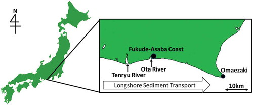
Figure 2. Map of Fukude-Asaba Coast, Shizuoka Prefecture, Japan. Pipeline-based sand bypassing system (indicated by the orange line) carries sediments from west to east with a design rate of 80 × 103 m3/year.
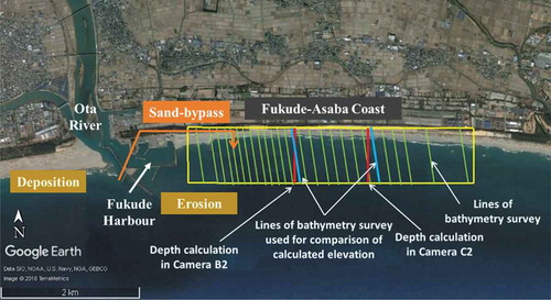
Figure 3. Rectified TIMEX image of eight cameras (top) and the bathymetry estimated by Okabe and Kato (Citation2017) by using fish finder log (bottom). The area is represented by the yellow rectangle in . The location of the outlet pipe of sand bypassing is indicated by the arrow. The red lines represent the cross-shore transects analyzed in this study.
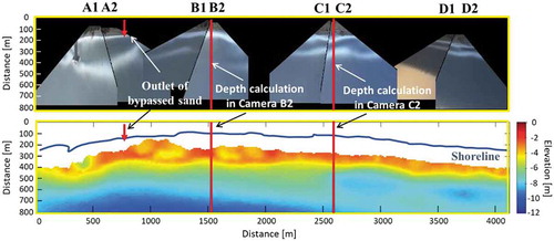
Figure 4. Method to calculate the rapid increase of brightness.
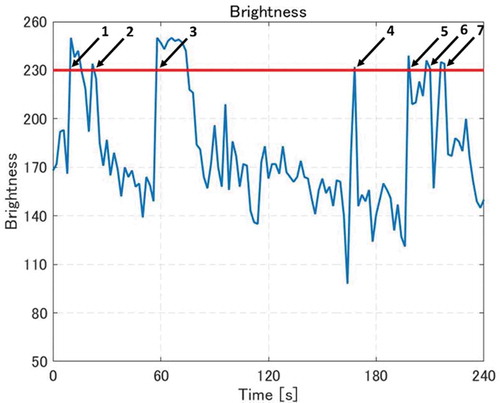
Figure 5. Shadow zone behind a breaking wave leading to the overestimation of wave breaking density. shows the depression angle, H shows the wave height, r shows the distance between the camera and the wave,
shows the height of the camera.
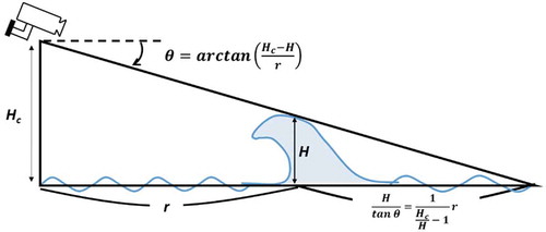
Figure 6. Relationship between the overestimation rate and the distance r from the camera. The overestimation of wave breaking density can be compensated by .
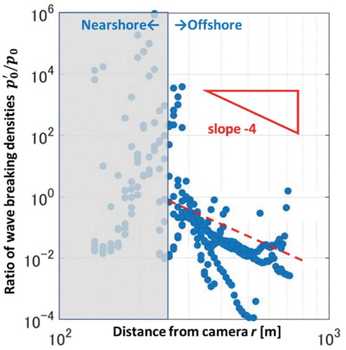
Figure 7. Change of wave height distribution before and after wave breaking. H shows the wave height and shows the mean wave height.
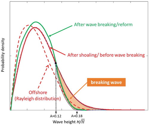
Figure 8. Change of wave height distribution and wave breaking density for an assumed topography.
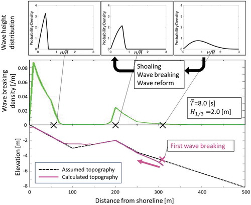
Figure 10. Wave conditions in October 2017 and the dates used to calculate water depth.
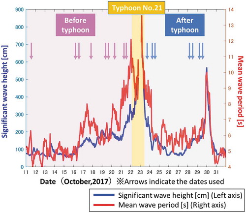
Figure 11. Rectified image of B2 Camera with the line used for the profile comparison.
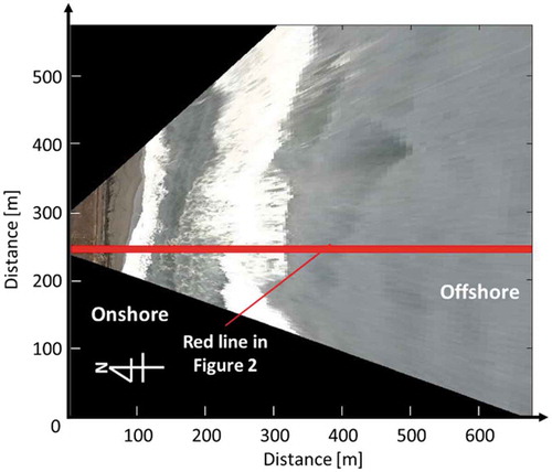
Figure 12. Estimated bathymetry before the typhoon (Camera B2).
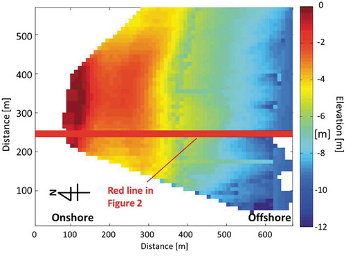
Figure 13. Nearshore profiles in the area covered by Camera B2 and C2. The bathymetry surveys were conducted in February 2017 and January 2018. Okabe’s data represent the bathymetry in the period from September 2016 to January 2017.
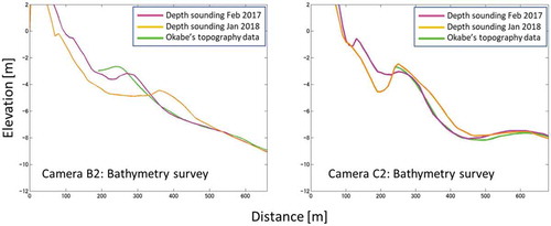
Figure 14. Time-averaged imageries for Camera B2 and C2.
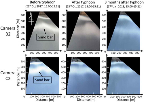
Figure 15. Coastal profile with wave breaking density for the area of Camera B2 before the typhoon in October 2017.
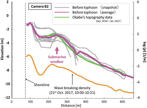
Figure 16. Coastal profile with wave breaking density for the area of Camera B2 after the typhoon in October 2017.
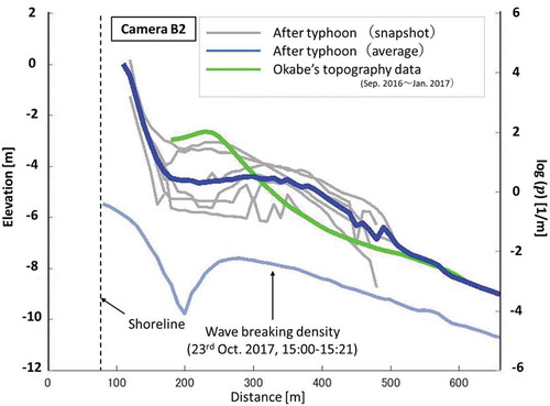
Figure 17. Comparison of bathymetries and wave breaking density before and after Typhoon No. 21.
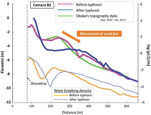
Figure 18. Comparison of profiles with depth sounding data in the area of Camera B2.
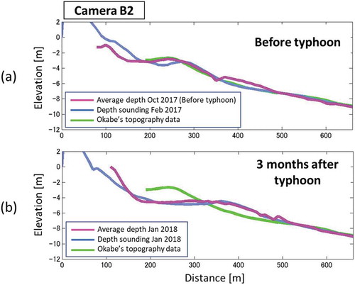
Figure 9. Topography calculation under different wave conditions ( is the mean wave period and
is the significant wave height).
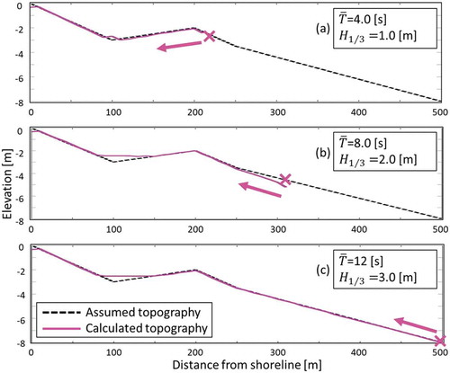
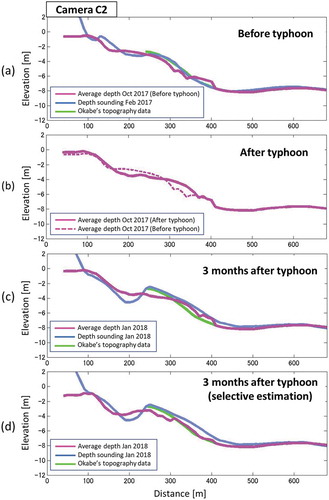
Figure 19. Bathymetry estimation using Camera C2. (a) Before typhoon (b) after the typhoon (c) 3 months after typhoon (d) 3 months after typhoon with selective averaging.