Ship-borne wave gauge using GNSS interferometric reflectometry

Figures & data

Figure 1. Schematic diagram of GNSS reflectometry.

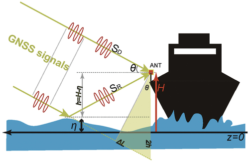
Figure 2. Simulated 20-Hz SNR variations for single-frequency waves $\mathit{h}$ with wave period T of 5 s and SWHs of 1.0 m (a) and 2.8 m (b). Horizontal lines at 2.25 dBhz (blue) and 1.0 dBhz (red) in panel (a) are drawn for the convenience of discussion in the text.

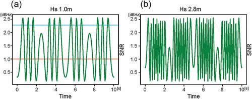
Figure 3. (a) Crossing number of simulated 20-Hz SNR over 10 s, Nc^10s, for single-frequency waves $\mathit{h}$ with different SWHs $H_S$ and wave periods $\mathit{T}$. Yellow, green and red curves represent results for wave periods of 2, 4, and 6 s, respectively. (b) Same as (a), but when counting duration is not fixed at 10 s but limited to the wave period $\mathit{T}$ in seconds, as $\mathit{N}{c}^T=\mathit{N}{c}^{10\mathrm{s}}\ast \mathit{T}/10\mathrm{s}$.

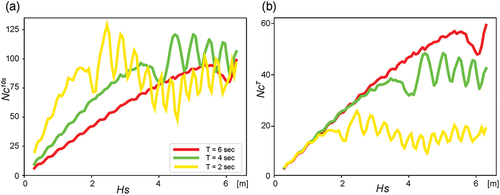
Figure 4. (a) Crossing number Nc^T for simulated 20-Hz SNR observations for single-frequency waves $\mathit{h}$ with a 6-s wave period and various SWHs $H_S$ and elevation angles $\mathit{\theta }$. Green, red, and blue curves represent results with elevation angles of 20°, 15° and 10°, respectively. (b) The same as (a), but when the crossing number Nc^T is normalized by $sin\mathit{\theta }$.

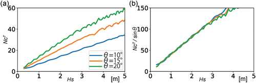
Figure 5. Period-averaged crossing number normalized by elevation angle $\mathit{\theta }$, $\mathit{N}{c}^{T_p}/sin\mathit{\theta }$, plotted for various SWHs and wave periods of multi-frequency waves with ISSC wave spectrum. The elevation angle $\mathit{\theta }$ is fixed at 18° as in Figure 3(b).

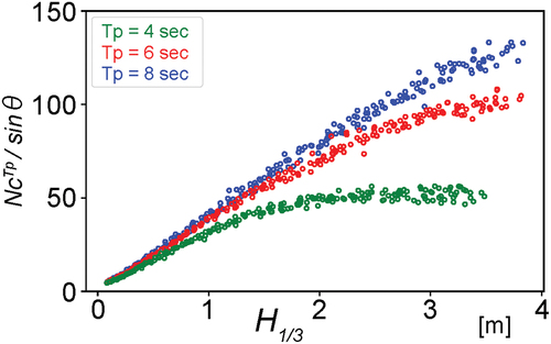
Figure 6. (a) GNSS antenna installed at starboard-side edge of New Camellia compass deck (yellow circle). (b) GNSS antenna (green circle) installed on edge of reflector metal plate overhanging seaward side of edge, which intentionally receives GNSS signals reflected from sea surface.

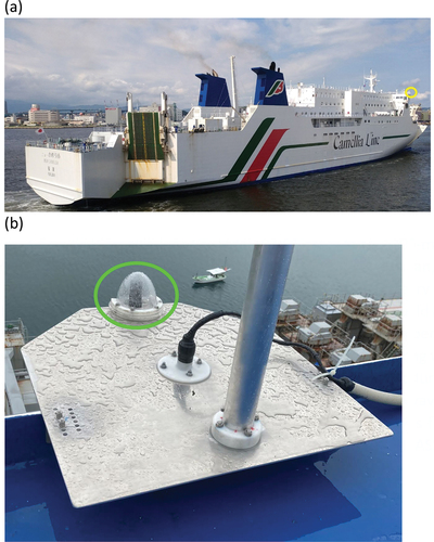
Table 1. Three cases for calibration of actual SNR observations, with the date in 2022, time in UTC, and locations. The wave periods and SWHs were obtained from JWA POLARIS hindcast data. For each case, two GNSS satellites used in the analysis are listed as sub-cases. For each sub-case, the satellite pseudo random noise code (PRN), elevation, and azimuth angles are shown, where the letters “G,” “R” and “C” stand for the GPS, GLONASS, and BeiDou satellites, respectively. The azimuth angle is measured clockwise from the ship heading (north-northwestward).

Case	Date	Time	Latitude [°N]	Longitude [°E]	SWH [m]	Period [s]	Sub-case	PRN	Elevation angle [°]	Azimuth angle [°]
1	5/18	14:10–14:12	34.196	129.926	0.17	3.6	1G	G08	12.9	103
							1R	R18	8.2	64
2	6/14	16:10–16:12	34.702	129.574	1.51	5.3	2G	G04	12.7	68
							2C	C33	7.6	44
3	6/24	14:10–14:12	34.138	129.951	2.56	6.4	3G	G03	13.8	44
							3R	R24	12.0	104

Figure 7. Example of actual 20-Hz observations of SNR variations. Data are for sub-case 1G (Table 1). The horizontal axis shows the elapsed time in seconds from 14:10 on 18 May 2022. The orange curve represents variations longer than 14 s, which could be induced by ship motion.

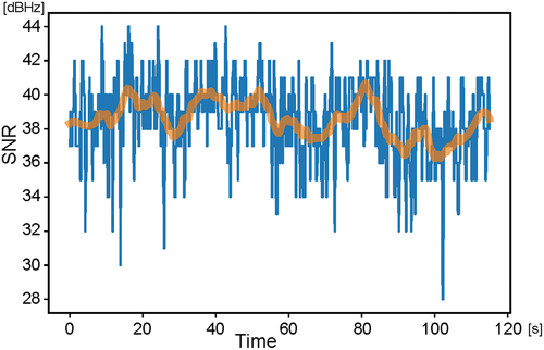
Figure 8. Schematic flow chart of present analysis.

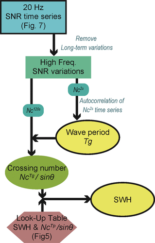
Figure 9. Temporal variations of crossing numbers within 2 s, $\mathit{N}{c}^{2\mathit{s}}$, for SNR records shown in Figure 7.

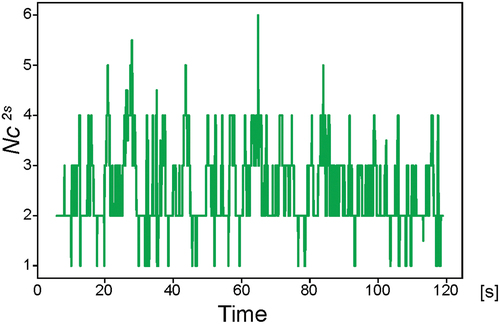
Figure 10. Results of comparisons for three cases. Red stars represent POLARIS hindcast data, and blue dots are the averages of the estimates of two sub-cases in each case (Table 1). Green numbers indicate cases, and blue letters show sub-cases.

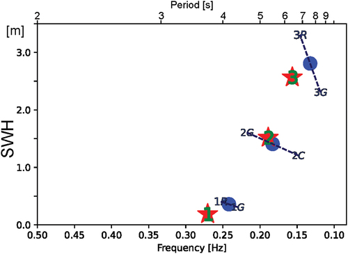
Table 2. Estimated SWH and wave period $T_g$ for each sub-case. Mean SWH and wave period are also listed for each case. The mean period is determined from the mean of the two frequencies. Due to differences in L1-band microwave wavelength $\mathit{\lambda }$ for satellites (0.1903 m for GPS; 0.1868 m for GLONASS; 0.1920 m for BeiDou), $\mathit{N}{c}^{T_g}$ values for GLONASS and BeiDou satellites have been modified by factors (1.02 and 0.99, respectively).

Case	Sub-case	Wave Period $T_g$ [s]		$\mathit{N}{c}^{T_g}/sin\mathit{\theta }$	SWH [m]
			mean			mean
1	1G	4.4	4.1	12.18	0.3	0.4
	1R	4.0		18.15	0.4
2	2G	4.6	5.5	60.72	1.6	1.4
	2C	6.8		49.51	1.2
3	3G	8.5	7.6	97.43	2.3	2.8
	3R	6.9		137.82	3.3