Characterising driver heterogeneity within stochastic traffic simulation

Figures & data

Figure 1. High-level schematic representation of the proposed framework. The top part refers to driver behaviour analysis; the lower part to driver behaviour simulation.

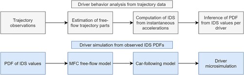
Figure 2. Identified sharp acceleration events corresponding to unconstrained vehicle movement in experimental observations.

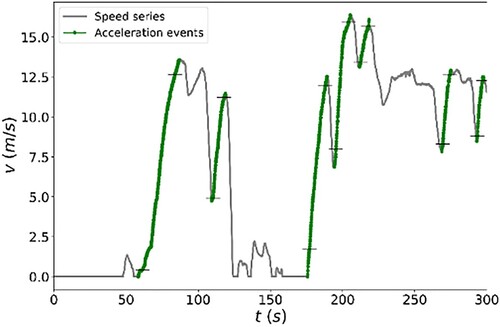
Figure 3. The unrealistic, feasible and common acceleration-speed domain [model representation from (He et al. 2020; Makridis et al. 2019)] for the vehicle used in the employed experimental campaign (see Section 2.4).

Figure 4. Naturalistic data refer to the 20 observed drivers of the experimental campaign used in this work. (a) shows acceleration over speed per movement and (b) the proposed $ds$ values per speed per movement.

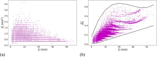
Figure 5. Uniform distribution of IDS values across the whole speed range. Data refer to 20 observed drivers ($\mathit{j}$ denotes the ID of an acceleration event).

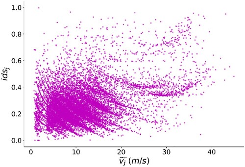
Table 1. Basic statistics of the trips per driver.

Driver	Total km	Total hours	Free-flow events number	Events (km)	Driver	Total km	Total hours	Free-flow events number	Events (km)
D1	250	8	715	117	D11	1056	14	420	171
D2	669	9	447	129	D12	119	4	456	55
D3	1973	39	2807	538	D13	1039	21	1401	307
D4	300	4	223	46	D14	1189	20	1009	295
D5	1055	14	482	134	D15	311	8	548	122
D6	45	2	176	20	D16	2581	35	942	405
D7	166	3	151	58	D17	288	7	632	118
D8	442	13	1054	150	D18	183	7	614	77
D9	310	7	619	111	D19	303	6	345	68
D10	174	6	481	71	D20	1424	19	1139	297

Figure 6. Histogram of the observed IDS values for each driver along with the fitted lognormal PDF. The vertical red lines denote the location of the median.

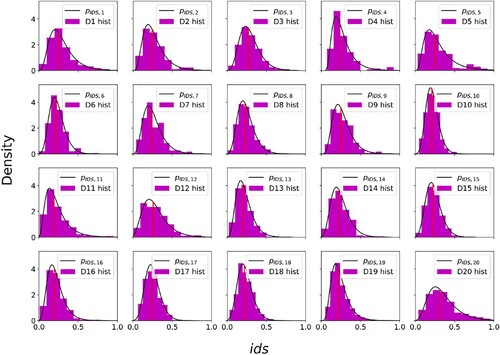
Figure 7. (a) K-means clustering result presented in a 3D plot, (b) PDFs of the inferred mild, normal and dynamic driver type.

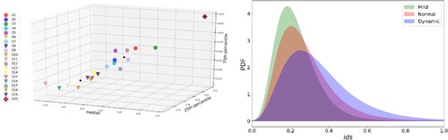
Figure 8. Bar plot of the IQR of the drivers’ PDFs.

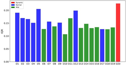
Figure 9. Reproduction of empirically-observed traffic oscillations with the MFC-LWR model as shown in (Makridis et al. 2020).

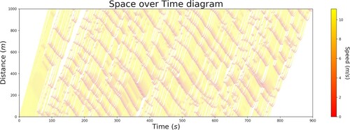
Figure 10. Median acceleration per event histograms of measured and simulated data.

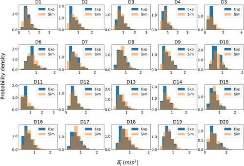
Figure 11. An indicative unconstrained movement per driver. For each event, the simulation area with the 25^th and 75th percentile from the driver’s PDF is highlighted.

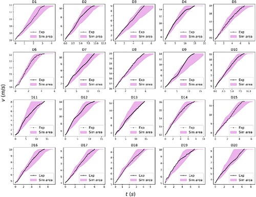
Figure 12. Histograms of median accelerations of the simulations concerning the three driver types.

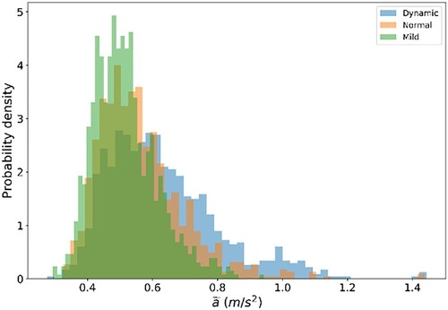
Table A1. Characteristics of fitted curves along with the special conditions for each one.

Curve	Polynomial curves	Special conditions
$f_{\text{min}}$	$f_{\text{min}}\left(\tilde{v}\right)=0.009\cdot \tilde{v}-0.009$	$f_{\text{min}}\left(\tilde{v}\right)\ge Min{\widetilde{ds}}_{exp}$
$f_{\text{max}}$	$f_{\text{max}}\left(\tilde{v}\right)=3.70\cdot {10}^{-5}{\tilde{v}}^3-0.003{\tilde{v}}^2+0.084\cdot \tilde{v}+0.167$

Table A2. The goodness of fit test results based on the K-S method.

Driver	Critical value	D statistic	p-value	Driver	Critical value	D statistic	p-value
D1	0.061	0.037	0.280	D11	0.080	0.019	0.999
D2	0.077	0.032	0.739	D12	0.076	0.036	0.596
D3	0.031	0.013	0.710	D13	0.043	0.019	0.662
D4	0.109	0.042	0.822	D14	0.051	0.032	0.264
D5	0.074	0.040	0.404	D15	0.070	0.023	0.928
D6	0.123	0.067	0.391	D16	0.053	0.035	0.188
D7	0.132	0.048	0.870	D17	0.065	0.026	0.768
D8	0.050	0.015	0.969	D18	0.066	0.024	0.859
D9	0.065	0.036	0.396	D19	0.088	0.035	0.782
D10	0.074	0.039	0.435	D20	0.048	0.022	0.662

Table A3. Parameters of the lognormal PDFs.

Driver	shape	location	scale	Driver	shape	location	scale
D1	0.448	−0.051	0.311	D11	0.560	−0.025	0.219
D2	0.456	−0.030	0.272	D12	0.383	−0.124	0.381
D3	0.312	−0.120	0.392	D13	0.355	−0.067	0.272
D4	0.529	0.031	0.208	D14	0.334	−0.099	0.324
D5	0.575	−0.011	0.258	D15	0.238	−0.182	0.405
D6	0.265	−0.132	0.353	D16	0.369	−0.068	0.267
D7	0.382	−0.064	0.300	D17	0.207	−0.211	0.452
D8	0.298	−0.113	0.340	D18	0.228	−0.189	0.409
D9	0.378	−0.046	0.295	D19	0.400	−0.026	0.244
D10	0.211	−0.166	0.375	D20	0.410	−0.089	0.405

He, Y., M. Makridis, K. Mattas, G. Fontaras, B. Ciuffo, and H. Xu. 2020. “Introducing Electrified Vehicle Dynamics in Traffic Simulation.” Transportation Research Record: Journal of the Transportation Research Board 2674: 776–791. doi:10.1177/0361198120931842.

 Web of Science ®Google Scholar

Makridis, M., G. Fontaras, B. Ciuffo, and K. Mattas. 2019. “MFC Free-Flow Model: Introducing Vehicle Dynamics in Microsimulation.” Transportation Research Record, 036119811983851. doi:10.1177/0361198119838515.

 Web of Science ®Google Scholar

Makridis, M., L. Leclercq, B. Ciuffo, G. Fontaras, and K. Mattas. 2020. “Formalizing the Heterogeneity of the Vehicle-driver System to Reproduce Traffic Oscillations.” Transportation Research Part C: Emerging Technologies 120: 102803.

 Web of Science ®Google Scholar