A fully automated pipeline of extracting biomarkers to quantify vascular changes in retina-related diseases

Figures & data

Figure 1. The pipeline for the analysis of retinal vascular biomarkers.

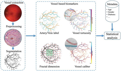
Figure 2. The whole routine of achieving elongated structure enhancement operation $\mathrm{{\rm Y}}$ via left-invariant operation $\mathrm{\Phi }$ based on the locally adaptive frame $\left\{{\mathrm{\partial }}_a,{\mathrm{\partial }}_b,{\mathrm{\partial }}_c\right\}$. The exponential curve fit provides the LAD frame with full alignment to local structures. An orientation score $U_f:={\mathcal{W}}_{\psi }f$ can be constructed from a 2D image $f$ to an orientation score $U_f$ via wavelet-type transform ${\mathcal{W}}_{\psi }$, where we choose cake wavelets (Bekkers et al. 2014b)) for $\psi$.

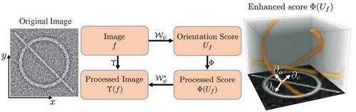
Figure 3. An example of the proposed optic disc (OD) and fovea detection. From Columns 1 to 5: original colour fundus image with manually annotated OD (black star) and fovea (white star), normalised green channel, Gaussian blurred image, PSEF response, and maximum response of PSEF indicating the OD location (red star) and the corresponding detected fovea (green star).

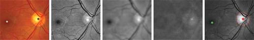
Table 1. The complete set of features extracted for each centreline pixel.

Category	Description	Index
Local intensities	The pixel intensity of normalised R, G, B, H, Sat., Bri., RG, MSR-R, MSR-G, MSR-RG, Ill.	F1 F11
Vessel width	The vessel width estimated at each pixel.	F12
Spatial coordinate	Euclidean distance to OD and image centre, angle with respect to OD.	F13 F15
Circular zone A	The mean, std, min, med and max of the 11 local intensities within a circular region with radius 0.5*vessel width.	F16 F70
Circular zone B	The mean, std, min, med and max of the 11 local intensities within a circular region with radius 1.0*vessel width.	F71 F125
Circular zone C	The mean, std, min, med, max of the 11 local intensities within a circular region with radius 2.0*vessel width.	F126 F180
Centrelines	The mean, std, min, med and max of the 11 local intensities along every centreline.	F181 F235
Vessel segments	The mean, std, min, med and max of the 11 local intensities within every vessel segment.	F236 F290
All centrelines	The mean, std, min, med and max of the 11 local intensities of all centreline pixels.	F291 F345
All vessel segments	The mean, std, min, med and max of the 11 local intensities of all vessel segment pixels.	F346 F400
Whole field of view	The mean, std, min, med and max of the 11 local intensities of all pixels inside the field of view.	F401 F455

Table 2. Segmentation results on the DRIVE and STARE data sets.

			DRIVE				STARE
	Methods	Year	Se	Sp	Acc	AUC	Se	Sp	Acc	AUC
	Second human observer		0.7760	0.9724	0.9472		0.8952	0.9384	0.9349
Unsupervised	Zhang et al. (2010)	2010	0.7120	0.9724	0.9382		0.7177	0.9753	0.9484
	You et al. (2011)	2011	0.7410	0.9751	0.9434		0.7260	0.9756	0.9497
	Fraz et al. (2012b)	2012	0.7152	0.9759	0.9430		0.7311	0.9680	0.9442
	Roychowdhury et al. (2015)	2015	0.7395	0.9782	0.9494^a	0.9672^a	0.7317	0.9842^a	0.9560	0.9673
	Azzopardi et al. (2015)	2015	0.7655	0.9704	0.9442	0.9614	0.7716	0.9701	0.9497	0.9563
	Yin et al. (2015)	2015	0.7246	0.9790^a	0.9403		0.8541^a	0.9419	0.9325
	Proposed LID	2016	0.7473	0.9764	0.9474	0.9517	0.7676	0.9764	0.9546	0.9614
	Proposed LAD	2016	0.7743^a	0.9725	0.9476	0.9636	0.7791^b	0.9758	0.9554	0.9748^a
Supervised	Lupa¸scu et al. (2010)	2010	0.7200		0.9597^b	0.9561
	Mar´in et al. (2011)	2011	0.7067	0.9801	0.9452	0.9588	0.6944	0.9819	0.9526	0.9769
	Fraz et al. (2012a)	2012	0.7406	0.9807	0.9480	0.9747^b	0.7548	0.9763	0.9534	0.9768
	Orlando et al. (2016)]	2016	0.7897^b	0.9684			0.7680	0.9738
	Li et al. (2016)	2016	0.7569	0.9816^b	0.9527	0.9738	0.7726	0.9844^b	0.9628^b	0.9879^b

^aBest values in comparison with the unsupervised methods; ^bbest values in comparison with the supervised methods.

Table 4. Comparisons of the success rate of the proposed framework for OD detection on all 1200 MESSIDOR images.

Methods	Success rates	Number of fails
PSEF Dashtbozorg et al. (2016b)	99.75%	3
Marin et al. (2015)	99.75%	3
Dashtbozorg et al. (2015)	99.83%	2
Bekkers et al. (2014a)	99.50%	6
Giachetti et al. (2013)	99.67%	4
Mendonc¸a et al. (2013)	99.75%	3
Aquino et al. (2012)	98.83%	14
Yu et al. (2012)	99.08%	11
Shijian (2011)	99.75%	3

Table 5. Success rate of the proposed framework for fovea detection on the MESSIDOR data set compared with other methods.

		Success rates
Methods	Number of images	$0.25r_{OD}$	$0.5r_{OD}$	$1r_{OD}$	$2r_{OD}$
PSEF - Dashtbozorg et al. (2016b)	1200	66.50%	93.75%	98.87%	99.58%
Kao et al. (2014)	1200			97.80%
Gegundez-Arias et al. (2013)	1200	93.92%	96.08%	96.92%	97.83%
Yu et al. (2011)	1200		95.00%
Niemeijer et al. (2009)	1200	93.50%	96.83%	97.92%
PSEF Dashtbozorg et al. (2016b)	1136	69.19%	95.86%	99.65%	99.91%
Aquino (2014)	1136	83.01%	91.28%	98.24%	99.56%
Giachetti et al. (2013)	1136			99.1%
Gegundez-Arias et al. (2013)	1136	76.23%	93.84%	98.24%	99.30%

Figure 4. Examples of A/V pixel-wise classifications by using different feature subsets. The last column shows the classifications using total 45 features including all the normalised intensities and the reflection features (Huang et al. (2017a)). Blue indicates veins and red indicates arteries.

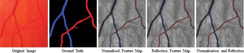
Figure 5. Two typical examples to show the vessel width-based artery and vein diameter ratio (AVR) difference in a specific ROI between one healthy subject and one diabetes type 2 subject. Blue indicates veins and red indicates arteries.

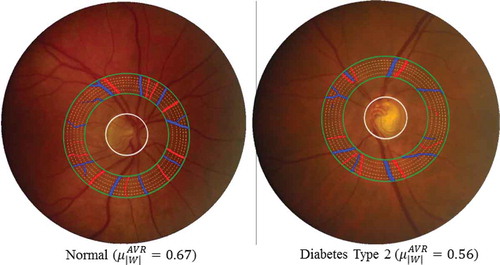
Figure 6. The stages of the proposed automatic width measurement technique: (a) centreline detection; (b) contour initialisation; (c) active contour segmentation; (d) obtaining the left and right edges; (e) Euclidean distance calculation; and (f) vessel calibre estimation.

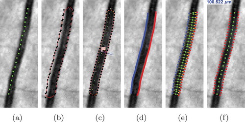
Figure 7. The vessels within the ROIs are used to compute the CRAE and CRVE values: (a) the widths of selected vessel are measured by the proposed method; (b) the six largest arteries and veins are then selected for the calculation of CRAE, CRVE and AVR values.

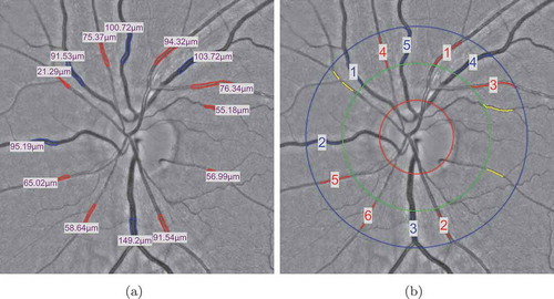
Figure 8. Validation of the $SE(2)$ exponential curvature estimation on a typical synthetic image. From left to right: input image (SNR = 1), ground truth colour-coded curvature map, measured curvature map with resp.

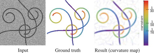
Figure 9. Examples to show the calculation of box dimension (BD) in a specific ROI between one healthy subject and one diabetes type 2 subject. Blue indicates veins and red indicates arteries.

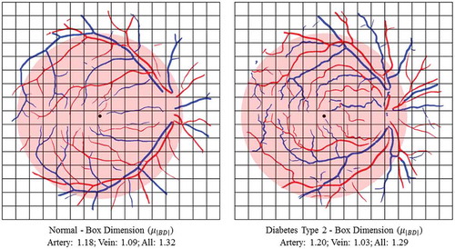
Figure 10. Examples of vessel segmentation by the proposed algorithm on images from the DRIVE and STARE data sets. Row 1: an image from the DRIVE data set ($Se=0.8329$, $Sp=0.9834$, $Acc=0.9656$ and $MCC=0.8324$). Row 2: an image from the STARE data set ($Se=0.8317$, $Sp=0.9792$, $Acc=0.9609$ and $MCC=0.8181$). From Columns 1 to 4: original colour images, vessel enhancement result, hard segmentation result and ground truth.

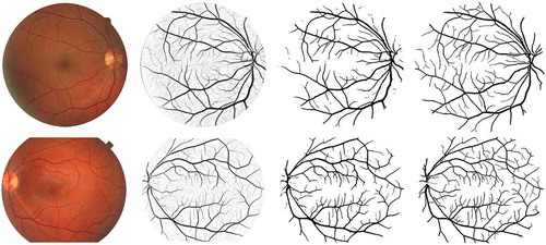
Figure 11. OD and fovea detection results and defined region of interest around OD or fovea centre.

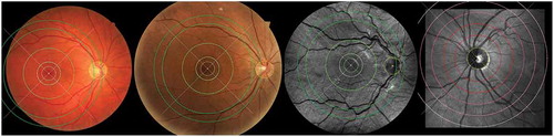
Table 3. The performance of the proposed framework on the DRIVE, INSPIRE, NIDEK, and Topcon data sets.

		Fovea-centred images					Optic disc-centred images
Data set	Resolution	$\mathrm{N}\mathrm{u}\mathrm{m}$	$Se$	$Acc$	$Sp$	$\mathrm{A}\mathrm{U}\mathrm{C}$	$\mathrm{N}\mathrm{u}\mathrm{m}$	$Se$	$Acc$	$Sp$	$\mathrm{A}\mathrm{U}\mathrm{C}$
DRIVE	565 $\times$ 584	20	72.0%	70.9%	73.8%	0.78
INSPIRE	2392 $\times$ 2048						20	90.2%	89.6%	91.3%	0.95
NIDEK	3744 $\times$ 3744	50	81.1%	81.3%	81.6%	0.89	50	83.6%	83.2%	84.9%	0.91
Canon	3456 $\times$ 2304	30	76.8%	77.8%	75.3%	0.84	30	78.3%	79.4%	76.1%	0.85
Topcon	2048 $\times$ 1536	30	82.5%	83.5%	81.8%	0.90	30	86.9%	87.6%	86.2%	0.93

Figure 12. A/V classification results from the DRIVE and INSPIRE data sets. From left to right: the original images, the A/V label of the vessel centrelines, the pixel-wise classification and the segment-wise classification. Correctly classified arteries are in red, correctly classified veins are in blue and the wrongly classified vessels are in yellow.

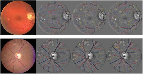
Figure 13. The Bland–Altman plots for comparing the (a) CRAE, (b) CRVE and (c) AVR values obtained by our method and the Vampire tool with the IVAN.

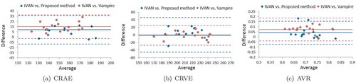
Figure 14. Two typical examples of showing the tortuosity (mean curvature) difference between one healthy subject and one diabetes type 2 subject. Blue indicates veins and red indicates arteries.

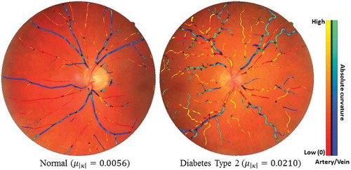
Table 8. The relative error of the CRAE, CRVE and AVR values obtained by the proposed method, IVAN and Vampire tools.

	Relative error
Software	CRAE	CRVE	AVR	Average
Our method	2.84%	2.40%	3.20%	2.81%
IVAN	2.32%	1.91%	2.65%	2.29%
Vampire	4.09%	3.63%	5.73%	4.48%

Table 6. Tortuosity measures ${\mu }_{\left|\kappa \right|}$ and ${\sigma }_{\left|\kappa \right|}$ in the MESSIDOR data set.

	Mean $\pm$ (STD)
Subgroup	${\mu }_{\left|\kappa \right|}({10}^{-2})$	${\sigma }_{\left|\kappa \right|}({10}^{-2})$
R0	1.624 $\pm$ (0.120)	2.333 $\pm$ (0.134)
R1	1.657 $\pm$ (0.124)	2.365 $\pm$ (0.131)
p-Value${ }^a$	0.007	0.020
R2	1.698 $\pm$ (0.122)	2.436 $\pm$ (0.144)
p-Value${ }^a$	$<$ 0.001	$<$ 0.001
R3	1.795 $\pm$ (0.160)	2.674 $\pm$ (0.235)
p-Value${ }^a$	$<$ 0.001	$<$ 0.001

^a Compared to R0.

Table 7. The mean and standard deviation of FD values ($D_B$) for different DR grades.

		ROI: full FOV			ROI: $5\times O{D}_R$
DR grade	Number	Mean	SD	RSD	Mean	SD	RSD
R0	546	1.3864	0.0324	2.34%	1.3285	0.0316	2.38%
R1	153	1.3852	0.0345	2.49%	1.3317	0.0304	2.28%
R2	247	1.3781	0.0364	2.64%	1.3215	0.0384	2.91%
R3	254	1.3869	0.0384	2.77%	1.3276	0.0375	2.82%
Total	1200	1.3846	0.0350	2.52%	1.3273	0.0343	2.59%

SD: standard deviation; RSD: relative standard deviation.

Table 9. Comparison between FD values in different DR groups.

			Mean	Std.		Confidence interval (95%)
DR grade			Difference	Error	p-Value^a	Lower bound	Upper bound
ROI: full FOV	R0	R1	.00123	.00319	.981	−.0070	.0094
		R2	.00834${ }^{\ast }$	.00267	.010	.0015	.0152
		R3	−.00046	.00265	.998	−.0073	.0063
	R1	R2	.00711	.00358	.195	−.0021	.0163
		R3	−.00169	.00356	.965	−.0109	.0075
	R2	R3	−.00879${ }^{\ast }$	.00311	.025	−.0168	−.0008
ROI: $5\times O{D}_R$	R0	R1	−.00324	.00313	.730	−.0113	.0048
		R2	.00696${ }^{\ast }$	.00263	.040	.0002	.0137
		R3	.00086	.00260	.987	−.0058	.0076
	R1	R2	.01020${ }^{\ast }$	.00352	.020	.0011	.0193
		R3	.00410	.00350	.646	−.0049	.0131
	R2	R3	−.00610	.00306	.191	−.0140	.0018
$$	$$	$$	$$	$$	$$	$$	$$

${ }^{\ast }$The mean difference is significant at the 0.05 level.

^aOne-way ANOVA test with null hypothesis that the means of distributions are equal.

Table 10. The comparison of FD between two human observers and the automated vessel segmentation method.

	Box dimension($D_B$)			Information dimension ($D_I$)			Correlation dimension($D_C$)
Method	Max^a	MRE^b	p-Value^c	Max	MRE	p-Value	Max	MRE	p-Value
Observer 2	7.1%	2.0%	0.0585	6.7%	1.9%	0.0851	6.2%	1.8%	0.0974
Zhang et al. (2015)	7.4%	3.9%	0.4950	7.4%	3.8%	0.8506	7.3%	3.8%	Â 0.691
Frangi et al. (1998)	9.3%	4.3%	0.8035	9.4%	4.3%	0.8802	9.4%	4.3%	Â 0.6990

^aMax: Maximum relative error with respect to Observer 1.

^bMRE: Mean of relative error with respect to Observer 1.

^cPearson correlation test with null hypothesis that the correlation coefficient is zero.

Table 11. The comparison of $D_B$ values using different region of interest.

Method	Radius	Max	MRE	p-Value${ }^{\ast }$
ROI1	$4\times O{D}_r$	3.8%	2.4%	$<0.01$
ROI2	$5\times O{D}_r$	1.0%	0.4%	$<0.01$
ROI3	$6\times O{D}_r$	Reference

${ }^{\ast }$Pearson correlation test with null hypothesis that the population correlation coefficient is zero with respect to ROI3.

Zhang B, Zhang L, Zhang L, Karray F. 2010. Retinal vessel extraction by matched filter with first-order derivative of Gaussian. Comput Biol Med. 40(4):438–445.

 PubMed Web of Science ®Google Scholar

You X, Peng Q, Yuan Y, Cheung Y-M, Lei J. 2011. Segmentation of retinal blood vessels using the radial projection and semi-supervised approach. Pattern Recogn. 44(10):2314–2324.

 Web of Science ®Google Scholar

Fraz MM, Barman SA, Remagnino P, Hoppe A, Basit A, Uyyanon-Vara B, Rudnicka AR, Owen CG. 2012b. An approach to localize the retinal blood vessels using bit planes and centerline detection. Comput Methods Programs Biomed. 108(2):600–616.

 PubMed Web of Science ®Google Scholar

Roychowdhury S, Koozekanani D, Parhi K. 2015. Iterative vessel segmentation of fundus images. IEEE Trans Biomed Eng. 62(7):1738–1749.

 PubMed Web of Science ®Google Scholar

Azzopardi G, Strisciuglio N, Vento M, Petkov N. 2015. Trainable COSFIRE filters for vessel delineation with application to retinal images. Med Image Anal. 19(1):46–57.

 PubMed Web of Science ®Google Scholar

Yin B, Huating L, Sheng B, Hou X, Chen Y, Wen W, Ping L, Shen R, Bao Y, Jia W. 2015. Vessel extraction from non-fluorescein fundus images using orientation-aware detector. Med Image Anal. 26(1):232–242.

 PubMed Web of Science ®Google Scholar

Lupa¸Scu CA, Tegolo D, Trucco E. 2010. FABC: retinal vessel segmentation using AdaBoost. IEEE Trans Inf Technol Biomed. 14(5):1267–1274.

 PubMed Web of Science ®Google Scholar

Mar´In D, Aquino A, Gegu´ndez-Arias ME, Bravo JM. 2011. A new supervised method for blood vessel segmentation in retinal images by using gray-level and moment invariants-based features. IEEE Trans Med Imag. 30(1):146–158.

 PubMed Web of Science ®Google Scholar

Fraz MM, Remagnino P, Hoppe A, Uyyanonvara B, Rudnicka AR, Owen CG, Barman SA. 2012a. An ensemble classification-based approach applied to retinal blood vessel segmentation. IEEE Trans Biomed Eng. 59(9):2538–2548.

 PubMed Web of Science ®Google Scholar

Orlando J, Prokofyeva E, Blaschko M. 2016. A discriminatively trained fully connected conditional random field model for blood vessel segmentation in fundus images. IEEE Trans Biomed Eng. PP(99):1–10. ISSN 0018-9294.

 Google Scholar

Li Q, Feng B, Xie L, Liang P, Zhang H, Wang T. 2016. A cross-modality learning approach for vesselsegmentation in retinal images. IEEE Trans Med Imag. 35(1): 109–118, Jan, ISSN 0278-0062

 PubMed Web of Science ®Google Scholar

Dashtbozorg B, Zhang J, Huang F, ter Haar Romeny BM. 2016b. Automatic optic disc and fovea detection in retinal images using super-elliptical convergence index filters. In: Campilho A, Karray, editors. Image analysis and recognition, volume 9730 of lecture notes in computer science. Cham, Switzerland: Springer; p. 697–706.

 Google Scholar

Marin D, Gegundez-Arias ME, Suero A, Bravo JM. 2015. Obtaining optic disc center and pixel region by automatic thresholding methods on morphologically processed fundus images. Comput Methods Programs Biomed. 118(2):173–185.

 PubMed Web of Science ®Google Scholar

Dashtbozorg B, Mendonc¸a AM, Campilho A. 2015. Optic disc segmentation using the sliding band filter. Comput Biol Med. 56:1–12.

 PubMed Web of Science ®Google Scholar

Bekkers RD, ter Haar Romeny B. 2014a. Optic nerve head detection via group correlations in multiorientation transforms. Lecture Notes Comput Sci. 8815:293–302.

 Google Scholar

Giachetti A, Ballerini L, Trucco E, Wilson PJ. 2013. The use of radial symmetry to localize retinal landmarks. Comput Med Imaging Graphics. 37(5):369–376.

 PubMed Web of Science ®Google Scholar

Mendonc¸a AM, Sousa A, Mendonc¸a L, Campilho A. 2013. Automatic localization of the optic disc by combining vascular and intensity information. Comput Med Imaging Graphics. 37(5):409–417.

 PubMed Web of Science ®Google Scholar

Aquino A, Gegundez ME, Marin D. 2012. Automated optic disc detection in retinal images of patients with diabetic retinopathy and risk of macular edema. Int J Biol Life Sci. 8(2):87–92.

 Google Scholar

Honggang Y, Simon Barriga E, Agurto C, Echegaray S, Pattichis MS, Bauman W, Soliz P. 2012. Fast localization and segmentation of optic disk in retinal images using directional matched filtering and level sets. IEEE Trans Inf Technol Biomed. 16(4):644–657.

 PubMedGoogle Scholar

Shijian L. 2011. Accurate and efficient optic disc detection and segmentation by a circular transformation. IEEE Trans Med Imaging. 30(12):2126–2133.

 PubMed Web of Science ®Google Scholar

Kao E-F, Lin P-C, Chou M-C, Jaw T-S, Liu G-C. 2014. Automated detection of fovea in fundus images based on vessel-free zone and adaptive Gaussian template. Comput Methods Programs Biomed. 117(2):92–103.

 PubMed Web of Science ®Google Scholar

Gegundez-Arias ME, Marin D, Bravo JM, Suero A. 2013. Locating the fovea center position in digital fundus images using thresholding and feature extraction techniques. Comput Med Imaging Graphics. 37(5):386–393.

 PubMed Web of Science ®Google Scholar

Yu H, Barriga S, Agurto C, Echegaray S, Pattichis M, Zamora G, Bauman W, Soliz P. 2011. Fast localization of optic disc and fovea in retinal images for eye disease screening. In:  Ronald M. Summers, Bram van Ginneken, editors, SPIE Medical Imaging. Lake Buena Vista(Orlando), FL: International Society for Optics and Photonics; p. 796317–796317.

 Google Scholar

Niemeijer M, Abr`Amoff MD, Van Ginneken B. 2009. Fast detection of the optic disc and fovea in color fundus photographs. Med Image Anal. 13(6):859–870.

 PubMed Web of Science ®Google Scholar

Aquino A. 2014. Establishing the macular grading grid by means of fovea centre detection using anatomicalbased and visual-based features. Comput Biol Med. 55:61–73.

 PubMed Web of Science ®Google Scholar

Huang F, Dashtbozorg B, ter Haar Romeny BM. 2017a. Artery/vein classification using reflection features in retina fundus images. Mach Vis Appl. 29(1): 1–12.

 Web of Science ®Google Scholar

Zhang J, Bekkers E, Abbasi S, Dashtbozorg B, ter Haar Romeny B. 2015. Robust and fast vessel segmentation via gaussian derivatives in orientation scores. In: Murino V, Puppo E, editors. Image analysis and processing, volume 9279 of lecture notes in computer science. Cham, Switzerland: Springer; p. 537–547.

 Google Scholar

Frangi A, Niessen W, Vincken K, Viergever M. Multiscale vessel enhancement filtering. In Medical Image Computing and Computer-Assisted Interventation (MICCAI 1998), 130–137. Springer, 1998.

 Google Scholar