VisionBlender: a tool to efficiently generate computer vision datasets for robotic surgery

Figures & data

Figure 1. VisionBlender’s user interface, displayed on the top right of the image

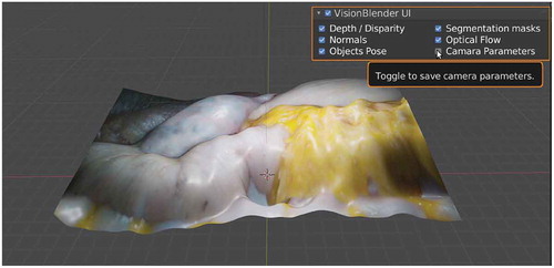
Figure 2. Example results of some generated ground truth maps in a video sequence of a robotic surgical instrument, moving over an ex vivo pig heart

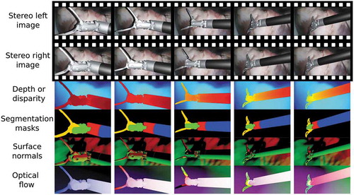
Table 1. An overview of render engines in Blender 2.82, which can be used to generate different ground truth maps

^aFor stereo images, VisionBlender generates disparity instead of depth maps.

Figure 3. Projecting the ray tracing distance $z^{\prime }$ into the orthogonal distance $z$

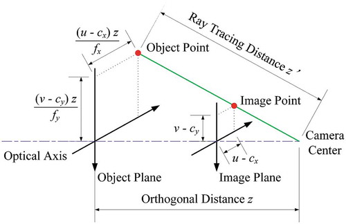
Figure 4. VisionBlender being used for training and validating an algorithm that estimates the pose of a surgical instrument using a cylindrical marker. This marker was taken from (Huang et al. 2020)

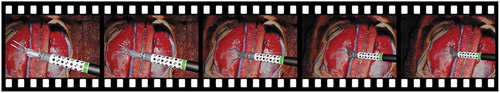
Figure 5. Example of a virtual scene – created after processing an input RGB-D image – illustrating a liver-stomach phantom. (c) shows the obtained virtual scene before any processing – for illustration purposes, the depth values of the holes were set to a large constant value, resulting in the visible ‘spikes’. (b) shows the virtual scene after filling 7,784 holes using (Liu et al. 2016), and (a), shows the resulting virtual scene after smoothing the tissue using Blender’s ‘CorrectiveSmooth‘ object modifier. Using (a) a user can generate an endoscopic dataset

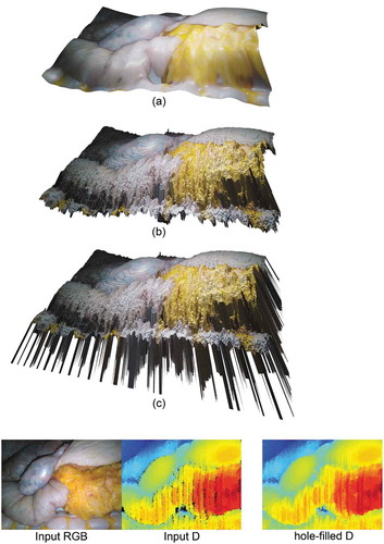
Figure 6. (a) Sample frames of our generated datasets including (1)-(2) training data from two different abdominal phantoms and testing data from an (3) ex vivo pig heart, and (4) ex vivo sheep brain. (b) Comparison example of the 3D reconstruction algorithms. (iv) is the left image from the stereo pair on which the ELAS algorithm had its best performance. (ii)-(iv) show the left-stereo images regenerated by using the disparity maps estimated with the supervised, unsupervised and ELAS algorithms, respectively. A colour map of the depth error is shown for each of the compared algorithms on the last column

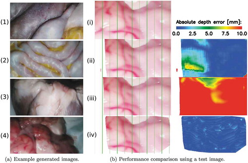
Table 2. Performance evaluation conducted on the test set, containing 1,000 stereo pairs of images. The table displays the mean and standard deviation values of the results on the test samples. For columns with red headers, a lower value is better. For the columns with green headers, higher value is better. The best performing model is highlighted in blue

Huang B, Tsai YY, Cartucho J, Vyas K, Tuch D, Giannarou S, Elson DS. 2020. Tracking and visualization of the sensing area for a tethered laparoscopic gamma probe. Int J Comput Assist Radiol Surg. 15(8):1389–1397. doi:10.1007/s11548-020-02205-z.

 Google Scholar

Liu S, Chen C, Kehtarnavaz N. 2016. A computationally efficient denoising and hole-filling method for depth image enhancement. In: Real-time image and video processing 2016. Vol. 9897, International Society for Optics and Photonics;SPIE Photonics Europe, 2016, Brussels, Belgium, p. 235–243. doi:10.1117/12.2230495.

 Google Scholar