Deep learning approach for hyperspectral image demosaicking, spectral correction and high-resolution RGB reconstruction

Figures & data

Figure 1. Examples to illustrate a hyperspectral cube as well as subsampling and demosaicking operations: (a) shows the spatial dimensions (X and Y) and spectral dimension of a hypercube; (b) shows how hyperspectral cube and snapshot mosaic images can be transformed into each other with band selection/spatial interpolation. Due to the space constraint of the image, $3\times 3$ snapshot mosaicking is taken as an example.

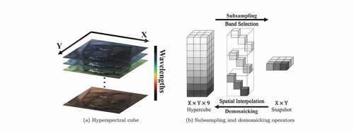
Figure 2. Diagram of the hyperspectral snapshot image demosaicking algorithm simulated using high-resolution line-scan data. The rectangular boxes contain the types of data as well as their corresponding shape, whereas the rounded boxes show the operations in each step. The blue boxes indicate the input and output of the algorithm.

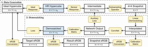
Figure 3. Comparison between the sRGB images converted from the ideal hyperspectral cube and demosaicked results from linear interpolation and supervised learning models.

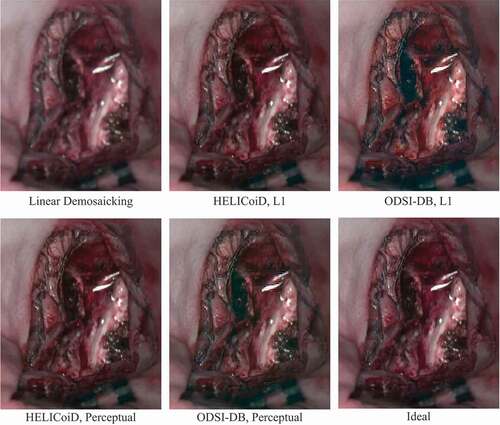
Figure 4. Percentage distribution of image quality scores in Likert scale given by the clinical experts.

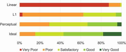
Figure 5. Preliminary test results on real snapshot data converted into sRGB images. The linear demosaicking and the proposed algorithm are compared. The two images on the right also illustrate oxygenation saturation maps derived from hyperspectral information.

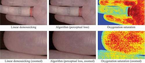
Table 1. Quantitative analysis of the demosaicked hyperspectral cubes from the HELICoiD and ODSI-DB hyperspectral datasets. The second row (L1 and Perceptual) refers to the choice of the auxiliary loss in the algorithm. The ODSI-DB $\to$ HELICoiD column indicates that the result is tested on the HELICoiD dataset using a network trained on the ODSI-DB dataset

	HELICoiD		ODSI-DB		ODSI-DB $\to$ HELICoiD
Eval\Train	L1	Perceptual	L1	Perceptual	L1	Perceptual
L1	$0.081\pm 0.036$	$\mathbf{0}\mathbf{.077}\pm \mathbf{0}\mathbf{.046}$	$0.023\pm 0.009$	$\mathbf{0}\mathbf{.018}\pm \mathbf{0}\mathbf{.007}$	$0.248\pm 0.104$	$\mathbf{0}\mathbf{.139}\pm \mathbf{0}\mathbf{.055}$
SSIM	$0.988\pm 0.006$	$\mathbf{0}\mathbf{.989}\pm \mathbf{0}\mathbf{.005}$	$\mathbf{0}\mathbf{.998}\pm \mathbf{0}\mathbf{.001}$	$\mathbf{0}\mathbf{.998}\pm \mathbf{0}\mathbf{.001}$	$0.946\pm 0.022$	$\mathbf{0}\mathbf{.959}\pm \mathbf{0}\mathbf{.019}$
PSNR	$37.4\pm 3.57$	$\mathbf{38}\mathbf{.3}\pm \mathbf{4}\mathbf{.25}$	$47.1\pm 3.26$	$\mathbf{49}\mathbf{.7}\pm \mathbf{3}\mathbf{.09}$	$27.2\pm 3.47$	$\mathbf{33}\mathbf{.6}\pm \mathbf{3}\mathbf{.03}$

Table 2. Perceptual metric scores on the sRGB images generated from the demosaicked hyperspectral cubes. All the results were tested on the HELICoiD dataset, and different demosaicking methods were compared (linear demosaicking, L1 model and perceptual model)

	HELICoiD			ODSI-DB $\to$ HELICoiD
sRGB Eval\Train	Linear	L1	Perceptual	L1	Perceptual
L1	$0.039\pm 0.008$	$0.012\pm 0.004$	$\mathbf{0}\mathbf{.011}\pm \mathbf{0}\mathbf{.002}$	$0.031\pm 0.010$	$\mathbf{0}\mathbf{.023}\pm \mathbf{0}\mathbf{.007}$
SSIM	$0.932\pm 0.021$	$0.975\pm 0.010$	$\mathbf{0}\mathbf{.979}\pm \mathbf{0}\mathbf{.008}$	$0.928\pm 0.026$	$\mathbf{0}\mathbf{.940}\pm \mathbf{0}\mathbf{.021}$
PSNR	$26.8\pm 1.57$	$34.8\pm 1.83$	$\mathbf{35}\mathbf{.1}\pm \mathbf{1}\mathbf{.56}$	$27.9\pm 2.18$	$\mathbf{29}\mathbf{.7}\pm \mathbf{2}\mathbf{.16}$
LPIPS	$0.209\pm 0.026$	$0.130\pm 0.018$	$\mathbf{0}\mathbf{.115}\pm \mathbf{0}\mathbf{.014}$	$0.199\pm 0.034$	$\mathbf{0}\mathbf{.178}\pm \mathbf{0}\mathbf{.036}$