Randomly connected neural networks for self-supervised monocular depth estimation

Figures & data

Figure 1. The proposed encoder-decoder architecture. The solid and the dotted lines denote forward propagation and skip connections, respectively. The purple lines signify the output left and right disparity maps generated at 4 scales, each increasing hierarchically with a scale factor of 2.

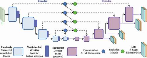
Figure 2. The process of generating a randomly connected deep-learning architecture. The red and the grey nodes are the input and the output nodes of the block, respectively. The black nodes are the convolution operations. The purple module is a multi-head self-attention module.

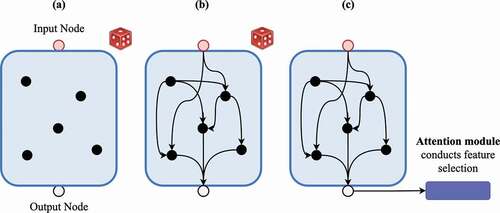
Figure 3. Showing the proposed learn-able skip connections methodology. $a$ is the network topology of a standard U-Net and $b$ is the proposed new network topology. Solid lines and dotted lines denote forward propagation and skip connections, respectively.

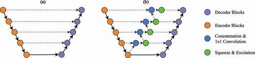
Figure 4. Discriminator model. The solid black lines and the dotted lines denote forward propagation and skip connections, respectively. The skip connection inputs are concatenated with the forward propagating feature map prior to being processed by the next layer. The pink lines show the extraction of multi-scale feature maps.

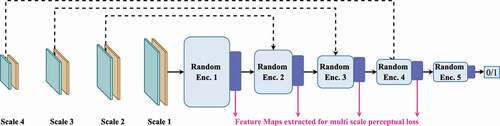
Figure 5. Depth maps generated by the proposed model on the SCARED and Hamlyn test splits shown in rows $A$ and $B$, respectively. Inclusion of $LS$ signifies presence of learn-able skip connections and $noLS$ without. All models were trained with the standard $L_{ssim}$ loss (Equation 1(1) $L_{ssim}={\delta }_1{L}_{recon}+{\delta }_2{L}_{smooth}+{\delta }_3{L}_{LRcons}$(1) ) unless $L_{Final}$ is specified, which signifies training with the proposed loss function (Equation 5(5) $\begin{array}{rl}& L_{final}={\delta }_1{L}_{recon}+{\delta }_2{L}_{smooth}+\\ & {\delta }_3{L}_{LRcons}+{\delta }_4{L}_{adv}^G+{\delta }_5{L}_{feat}\end{array}$(5) ). The colour bar displays the depth range in mm.

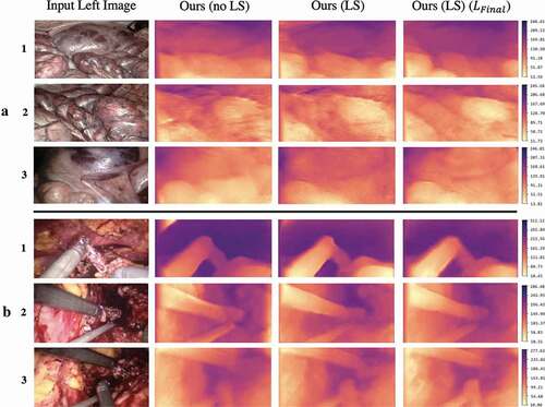
Figure 6. Comparison of depth maps generated by our model with Godard et al. (2017) and Pilzer et al. (2018) on the Hamlyn test split. The last column re-displays the depth produced by our proposed method (column 2), with the green boxes highlighting the key areas where more details are visible in our depth maps. The colour bar displays the depth range in mm.

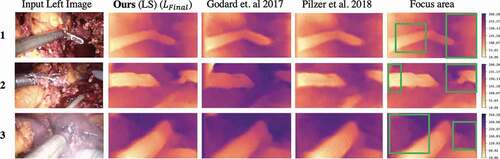
Table 1. Showing the mean absolute depth error in mm for test dataset 1 from SCARED. The compared methods are the self-supervised methods submitted to this challenge. (M) signifies Monodepth method and (S) Stereodepth. The presence of $L$ denotes the type of loss function used for training, and presence of (no LS) implies no learn-able skip connections were used in the model. Best results are highlighted in bold

Method	Keyframe 1	Keyframe 2	Keyframe 3	Keyframe 4	Keyframe 5	Average
Ours $L_{final}$ (M)	34.18 $\pm$ 0.071	27.01 $\pm$ 0.096	14.82 $\pm$ 0.063	13.42 $\pm$ 0.055	12.89 $\pm$ 0.067	20.46
Ours $L_{ssim}$ (M)	33.21 $\pm$ 0.069	26.73 $\pm$ 0.099	15.47 $\pm$ 0.066	15.13 $\pm$ 0.058	13.01 $\pm$ 0.066	20.71
Ours $L_{ssim}$ (no LS) (M)	35.02 $\pm$ 0.074	28.10 $\pm$ 0.091	16.89 $\pm$ 0.061	17.76 $\pm$ 0.061	13.26 $\pm$ 0.068	22.206
KeXue Fu (S)	30.49	18.32	19.73	19.30	16.86	20.94
Xiaohong Li (S)	34.42	20.66	17.84	27.92	13.00	22.77

Table 2. Showing the mean absolute depth error in mm for test dataset 2 from SCARED. The compared methods are the self-supervised methods submitted to this challenge. Where (M) signifies Monodepth method and (S) Stereodepth. The presence of $L$ denotes the type of loss function used for training, and presence of (no LS) implies no Learn-able skip connections were used in the model. Best results are highlighted in bold

Method	Keyframe 1	Keyframe 2	Keyframe 3	Keyframe 4	Keyframe 5	Average
Ours $L_{final}$ (M)	29.00 $\pm$ 0.061	25.81 $\pm$ 0.092	18.72 $\pm$ 0.064	8.90 $\pm$ 0.070	10.12 $\pm$ 0.044	18.51
Ours $L_{ssim}$ (M)	27.69 $\pm$ 0.059	26.17 $\pm$ 0.091	20.14 $\pm$ 0.061	9.11 $\pm$ 0.068	11.79 $\pm$ 0.054	18.98
Ours $L_{ssim}$ (no LS) (M)	28.25 $\pm$ 0.066	27.36 $\pm$ 0.088	22.83 $\pm$ 0.065	11.69 $\pm$ 0.073	13.51 $\pm$ 0.055	20.73
KeXue Fu (S)	23.71	15.46	26.43	9.60	10.92	17.22
Xiaohong Li (S)	24.58	16.80	29.92	11.37	19.93	20.52

Table 3. SSIM index on the reconstructed images generated via the estimated disparity maps on the Hamlyn test dataset. Higher value indicates better performance. Where (M) signifies Monodepth method and (S) Stereodepth. The M in parameter count signifies a million parameters. Methods $A$,$B$,$C$,$D$ and $E$ are Geiger et al. (2010), Yamaguchi et al. (2014), Ye et al. (2017), Godard et al. (2017) and Pilzer et al. (2018), respectively

Method	A (S)	B (S)	C (S)	D (M)	E (S)	Ours (M)
Mean SSIM	0.473	0.547	0.604 $\pm$ 0.066	0.611 $\pm$ 0.076	0.633 $\pm$ 0.079	0.672 $\pm$ 0.080
Parameter count	–	–	32 M	31 M	31 M	22 M

Godard C, Mac Aodha O, Brostow GJ. 2017. Unsupervised monocular depth estimation with left-right consistency. In: IEEE Conference on Computer Vision and Pattern Recognition (CVPR), Honolulu, Hawaii.

 Google Scholar

Pilzer, Andrea, Dan Xu, Mihai Marian Puscas, Elisa Ricci and N. Sebe. 2018. “Unsupervised Adversarial Depth Estimation Using Cycled Generative Networks.” 2018 International Conference on 3D Vision (3DV) : 587–595.

 Google Scholar

Geiger A, Roser M, Urtasun R. 2010. Efficient large-scale stereo matching. ACCV. Berlin, Heidelberg: Springer

 Google Scholar

Yamaguchi K, McAllester DA, Urtasun R 2014. Efficient joint segmentation, occlusion labeling, stereo and flow estimation. In: ECCV,  Zurich, Switzerland.

 Google Scholar

Ye M, Johns E, Handa A, Zhang L, Pratt P, Yang G 2017. Self-supervised siamese learning on stereo image pairs for depth estimation in robotic surgery. ArXiv. abs/1705.08260.

 Google Scholar