A Multi-View Semi-supervised learning method for knee joint cartilage segmentation combining multiple feature descriptors and image modalities

Figures & data

Figure 1. General flowchart of the proposed method.

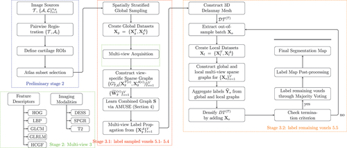
Figure 2. Each atlas ${\mathcal{A}}_i$ is affinely registered to the target image $\mathcal{T}$, and the obtained transformation is subsequently applied to the corresponding masks ${\mathcal{L}}_i$. A majority voting filter (MV) produces an initial pre-segmentation mask $({\tilde{\mathcal{L}}}^{\mathcal{T}})$ of cartilage-only labels and the Region of Interest (ROI) is finally defined as the morphological dilation of ${\tilde{\mathcal{L}}}^{\mathcal{T}}$.

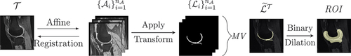
Figure 3. Schematic representation of the feature description process for a regional SV ${\mathcal{R}}_i$, centered around a voxel ${\mathbf{x}}_i$. Each SV comprises $3\times 3\times 3$ patches, which in turn consist of $5\times 5\times 5$ voxels. For all patches ${\mathbf{p}}_{\mathbf{j}}^{\mathbf{(}\mathbf{i}\mathbf{)}}\in {\mathcal{R}}_i$, a feature vector ${\mathbf{h}}_j^{(i)}$ is calculated according to an encoding function (HOG, LBP, etc.), here denoted as $f_{\mathit{enc}}(\cdot )$, where ${\mathbf{h}}_j^{(i)}$ serves as the individual descriptor for ${\mathbf{p}}_j^{(i)}$. Finally, the whole ${\mathcal{R}}_i$ is characterized by ${\mathbf{H}}_i$ as the weighted aggregation of all its constituent descriptors.

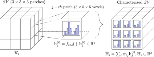
Table 1. Displacement vectors for GLCM and GLRLM for volumetric data.

Direction	Displacement Vector
$(0,\mathit{\pi }/2)$	$(\mathit{d},0,0)$
$(\mathit{\pi }/4,\mathit{\pi }/2)$	$(\mathit{d},\mathit{d},0)$
$(\mathit{\pi }/2,\mathit{\pi }/2)$	$(0,\mathit{d},0)$
$(3\mathit{\pi }/4,\mathit{\pi }/2)$	$(-\mathit{d},\mathit{d},0)$
$(\cdot ,0)$	$(0,0,\mathit{d})$
$(0,\mathit{\pi }/4)$	$(\mathit{d},0,\mathit{d})$
$(\mathit{\pi }/4,\mathit{\pi }/2-arcsin\sqrt{1/3}$	$(\mathit{d},\mathit{d},\mathit{d})$
$(\mathit{\pi }/2,\mathit{\pi }/4)$	$(0,\mathit{d},\mathit{d})$
$(3\mathit{\pi }/4,\mathit{\pi }/2-arcsin\sqrt{1/3})$	$(-\mathit{d},\mathit{d},\mathit{d})$
$(0,3\mathit{\pi }/4)$	$(\mathit{d},0,-\mathit{d})$
$(\mathit{\pi }/4,\mathit{\pi }/2-arcsin\sqrt{1/3})$	$(\mathit{d},\mathit{d},-\mathit{d})$
$(\mathit{\pi }/2,3\mathit{\pi }/4)$	$(0,\mathit{d},-\mathit{d})$
$(3\mathit{\pi }/4,arcsin\sqrt{1/3})$	$(-\mathit{d},\mathit{d},-\mathit{d})$

Figure 4. Schematic representation of multi-view feature extraction for regional SV ${\mathcal{R}}_i$. Each one of the $\mathit{j}=1,\cdots ,27$ patches is supplied with a feature vector for each descriptor(view) employed. The regional feature vector for each view is then calculated according to the process outlined in Figure 3. The overall description of ${\mathcal{R}}_i$ is the collection of all $\{{\mathbf{H}}_{\mathbf{i}}^{\mathbf{(}\mathbf{v}\mathbf{)}}{\}}_{v=1}^{\mathcal{V}}$.

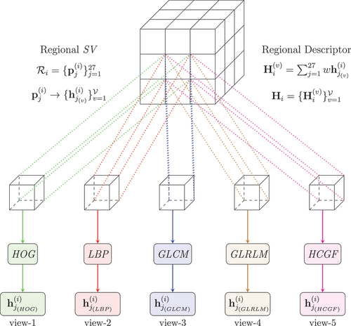
Figure 5. DESS, SPGR and T2 MRI sequences for the same subject. The differences in intensity profiles is apparent, especially between sequence T2 and the rest, suggesting that features learned from these images will yield sufficiently different descriptions of the image information content.

Figure 6. Out-of-sample label propagation: two sparse graphs ${\tilde{\mathbf{W}}}_{\mathit{og}}^{(\mathit{v})},{\tilde{\mathbf{W}}}_{\mathit{ol}}^{(\mathit{v})}$ are constructed for each view $\mathit{v}$ of the out-of-sample batch ${\mathbf{X}}_o^{(v)}$, connecting it to the global ${\mathbf{X}}_g^{(v)}$ and local ${\mathbf{X}}_l^{(v)}$ datasets respectively. The multi-view coefficients $\mathit{\alpha }$ are used to yield the final learned sparse graphs facilitating the labelling of voxels in ${\mathbf{X}}_o$.

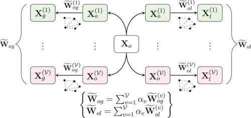
Table 2. Test cases examined for the first group of experiments.

	Descriptor
	HOG	LBP	GLCM	GLRLM	HCGF
Case 1	✓
Case 2	✓	✓
Case 3	✓	✓	✓	✓
Case 4	✓	✓	✓	✓	✓

Figure 7. Effect of number of atlases on $\mathit{DSC}$ score.

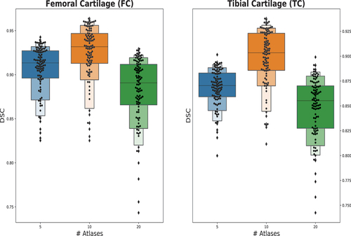
Figure 8. Effect of amount of supervision on $\mathit{DSC}$ score.

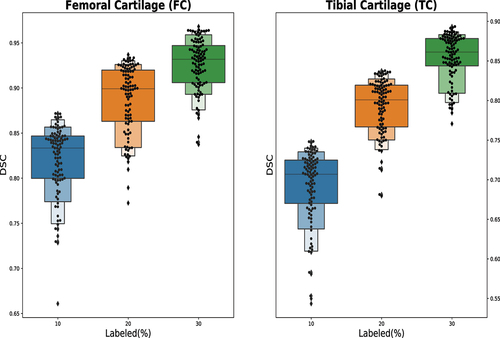
Figure 9. Effect of number of sparse neighbors on $\mathit{DSC}$ score.

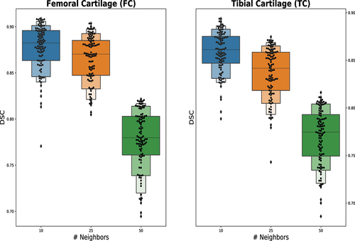
Figure 10. Effect of structural regularization parameter on $\mathit{DSC}$ score.

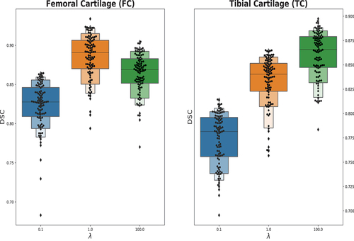
Figure 11. Effect of convex combination parameter on $\mathit{DSC}$ score.

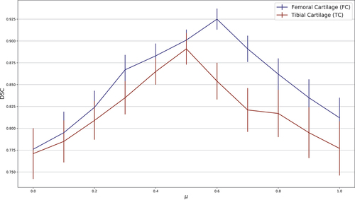
Table 3. Performance comparison (mean and std. deviations) of all test cases for the proposed method of MV-HyLP. In case #1, GLM denotes the combination of GLCM, GLLM and All, the inclusion of all feature descriptors. Stacked and fused in case #2 refer to the list of feature descriptors (HOG, LBP, HCGF) being concatenated and fused through AMUSE, respectively. Finally, in case #3, Multi-feature corresponds exactly to the last row in case #1.

		Femoral Cartilage					Tibial Cartilage
Method	Case	Recall	Precision	DSC	VOE	VD	Recall	Precision	DSC	VOE	VD
Group #1	HOG	$88.81\mathrm{\%}$	$88.17\mathrm{\%}$	$88.56\mathrm{\%}$	$23.19\mathrm{\%}$	$6.02\mathrm{\%}$	$85.72\mathrm{\%}$	$83.91\mathrm{\%}$	$84.03\mathrm{\%}$	$27.13\mathrm{\%}$	$9.09\mathrm{\%}$
		$(\pm 0.212)$	$(\pm 0.227)$	$(\pm 0.191)$	$(\pm 0.208)$	$(\pm 0.265)$	$(\pm 0.176)$	$(\pm 0.134)$	$(\pm 0.162)$	$(\pm 0.207)$	$(\pm 0.181)$
	HOG+LBP	$91.97\mathrm{\%}$	$90.40\mathrm{\%}$	$89.67\mathrm{\%}$	$22.35\mathrm{\%}$	$6.02\mathrm{\%}$	$85.88\mathrm{\%}$	$85.36\mathrm{\%}$	$85.79\mathrm{\%}$	$25.29\mathrm{\%}$	$7.79\mathrm{\%}$
		$(\pm 0.055)$	$(\pm 0.049)$	$(\pm 0.029)$	$(\pm 0.035)$	$(\pm 0.038)$	$(\pm 0.046)$	$(\pm 0.27)$	$(\pm 0.021)$	$(\pm 0.033)$	$(\pm 0.016)$
	HOG+LBP+GLM	$92.24\mathrm{\%}$	$89.76\mathrm{\%}$	$90.37\mathrm{\%}$	$21.34\mathrm{\%}$	$5.84\mathrm{\%}$	$86.89\mathrm{\%}$	$87.75\mathrm{\%}$	$86.54\mathrm{\%}$	$24.54\mathrm{\%}$	$6.67\mathrm{\%}$
		$(\pm 0.052)$	$(\pm 0.051)$	$(\pm 0.026)$	$(\pm 0.028)$	$(\pm 0.034)$	$(\pm 0.047)$	$(\pm 0.023)$	$(\pm 0.018)$	$(\pm 0.025)$	$(\pm 0.011)$
	All	$93.24\mathrm{\%}$	$91.26\mathrm{\%}$	$91.76\mathrm{\%}$	$20.65\mathrm{\%}$	$5.17\mathrm{\%}$	$90.89\mathrm{\%}$	$89.79\mathrm{\%}$	$88.65\mathrm{\%}$	$22.95\mathrm{\%}$	$6.05\mathrm{\%}$
		$(\pm 0.052)$	$(\pm 0.051)$	$(\pm 0.026)$	$(\pm 0.028)$	$(\pm 0.034)$	$(\pm 0.047)$	$(\pm 0.023)$	$(\pm 0.018)$	$(\pm 0.025)$	$(\pm 0.011)$
Group #2	Stacked	$88.70\mathrm{\%}$	$90.10\mathrm{\%}$	$89.56\mathrm{\%}$	$21.95\mathrm{\%}$	$55.90\mathrm{\%}$	$76.12\mathrm{\%}$	$80.90\mathrm{\%}$	$85.43\mathrm{\%}$	$5.16\mathrm{\%}$	$29.05\mathrm{\%}$
		$(\pm 0.195)$	$(\pm 0.214)$	$(\pm 0.158)$	$(\pm 0.223)$	$(\pm 0.144)$	$(\pm 0.098)$	$(\pm 0.117)$	$(\pm 0.154)$	$(\pm 0.174)$	$(\pm 0.139)$
	Fused	$77.90\mathrm{\%}$	$87.30\mathrm{\%}$	$90.67\mathrm{\%}$	$12.00\mathrm{\%}$	$29.97\mathrm{\%}$	$91.50\mathrm{\%}$	$93.60\mathrm{\%}$	$87.12\mathrm{\%}$	$86.20\mathrm{\%}$	$11.18\mathrm{\%}$
		$(\pm 0.098)$	$(\pm 0.089)$	$(\pm 0.045)$	$(\pm 0.038)$	$(\pm 0.063)$	$(\pm 0.038)$	$(\pm 0.041)$	$(\pm 0.057)$	$(\pm 0.061)$	$(\pm 0.044)$
Group #3	Multi-Modal	$90.02\mathrm{\%}$	$90.71\mathrm{\%}$	$89.93\mathrm{\%}$	$18.96\mathrm{\%}$	$5.85\mathrm{\%}$	$85.49\mathrm{\%}$	$87.59\mathrm{\%}$	$87.31\mathrm{\%}$	$8.78\mathrm{\%}$	$21.76\mathrm{\%}$
		$(\pm 0.232)$	$(\pm 0.247)$	$(\pm 0.191)$	$(\pm 0.218)$	$(\pm 0.241)$	$(\pm 0.168)$	$(\pm 0.137)$	$(\pm 0.185)$	$(\pm 0.202)$	$(\pm 0.153)$
	All	$94.04\mathrm{\%}$	$93.16\mathrm{\%}$	$92.56\mathrm{\%}$	$15.16\mathrm{\%}$	$5.12\mathrm{\%}$	$91.08\mathrm{\%}$	$89.98\mathrm{\%}$	$89.91\mathrm{\%}$	$19.67\mathrm{\%}$	$5.85\mathrm{\%}$
		$(\pm 0.052)$	$(\pm 0.051)$	$(\pm 0.026)$	$(\pm 0.028)$	$(\pm 0.034)$	$(\pm 0.047)$	$(\pm 0.023)$	$(\pm 0.018)$	$(\pm 0.025)$	$(\pm 0.011)$

Figure 12. Segmentation results for femoral (FC) and tibial (TC) cartilage for the four instances of case #1 (left to right: Ground Truth, HOG, HOG & LBP, HOG & LBP & GLCM, all features). The first part of the figure illustrates a case of successful application of MV-KCS, while the second part presents in instance characterized by poor performance. In both cases, however, the positive effect of incorporating additional views is noticeable.

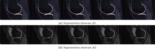
Table 4. Pairwise comparisons using the Nemenyi test for the cartilage $\mathit{DSC}$ results of the test cases in Table 3. Reported are the corresponding $\mathit{p}$-values. The binary indices in the subscript of each method’s name MV-HyLP_xxxxx indicate the inclusion or exclusion of the respective feature descriptor HOG, LBP, GLCM, GLRLM, HCGF..

	MV-HyLP10000	MV-HyLP11000	MV-HyLP11110
MV-HyLP11000	$2.81\times {10}^{-03}$	-	-
MV-HyLP11110	$1.05\times {10}^{-05}$	$3.75\times {10}^{-03}$	-
MV-HyLP11111	$4.28\times {10}^{-05}$	$2.25\times {10}^{-04}$	$1.13\times {10}^{-02}$

Table 5. Summary of segmentation performance measures (means and std. deviations) on the two cartilage classes of our proposed method MV-RegLP and its modification MV-HyLP, compared to Patch-Based Sparse-Coding (PB_SC), Patch-Based Sparse-Coding with stacked features (PB_SC^(stacked)), Patch-Based joint label fusion (PB-JLF), Triplanar CNN, SegNet, MM-CNN-FC, VoxResNet, DenseVoxNet, KCB-Net, CAN3D, 3D-CNN + SSM, DAN, UA-MT and SS-DTC. The hyperparameter values for MV-RegLP and MV-HyLP are those obtained after parameter sensitivity analysis in previous section 8.3.

	Femoral Cartilage					Tibial Cartilage
Method	Recall	Precision	$\mathit{DSC}$	$\mathit{VOE}$	$\mathit{VD}$	Recall	Precision	$\mathit{DSC}$	$\mathit{VOE}$	$\mathit{VD}$
PBSC	$83.51\mathrm{\%}$	$82.65\mathrm{\%}$	$82.23\mathrm{\%}$	$29.97\mathrm{\%}$	$11.01\mathrm{\%}$	$79.76\mathrm{\%}$	$81.45\mathrm{\%}$	$78.85\mathrm{\%}$	$34.28\mathrm{\%}$	$11.79\mathrm{\%}$
	$(\pm 0.065)$	$(\pm 0.042)$	$(\pm 0.047)$	$(\pm 0.062)$	$(\pm 0.074)$	$(\pm 0.033)$	$(\pm 0.022)$	$(\pm 0.021)$	$(\pm 0.044)$	$(\pm 0.043)$
PBSC^(stacked)	$84.12\mathrm{\%}$	$84.67\mathrm{\%}$	$84.35\mathrm{\%}$	$26.96\mathrm{\%}$	$7.35\mathrm{\%}$	$82.84\mathrm{\%}$	$83.67\mathrm{\%}$	$81.91\mathrm{\%}$	$30.12\mathrm{\%}$	$10.92\mathrm{\%}$
	$(\pm 0.068)$	$(\pm 0.041)$	$(\pm 0.044)$	$(\pm 0.062)$	$(\pm 0.078)$	$(\pm 0.039)$	$(\pm 0.016)$	$(\pm 0.027)$	$(\pm 0.033)$	$(\pm 0.034)$
PB-JLF	$84.61\mathrm{\%}$	$85.03\mathrm{\%}$	$84.92\mathrm{\%}$	$26.21\mathrm{\%}$	$7.28\mathrm{\%}$	$83.15\mathrm{\%}$	$83.92\mathrm{\%}$	$82.37\mathrm{\%}$	$29.41\mathrm{\%}$	$9.84\mathrm{\%}$
	$(\pm 0.102)$	$(\pm 0.065)$	$(\pm 0.081)$	$(\pm 0.104)$	$(\pm 0.092)$	$(\pm 0.061)$	$(\pm 0.048)$	$(\pm 0.036)$	$(\pm 0.067)$	$(\pm 0.041)$
Triplanar CNN	$85.04\mathrm{\%}$	$85.27\mathrm{\%}$	$84.98\mathrm{\%}$	$25.77\mathrm{\%}$	$7.11\mathrm{\%}$	$83.44\mathrm{\%}$	$84.07\mathrm{\%}$	$83.19\mathrm{\%}$	$28.96\mathrm{\%}$	$8.41\mathrm{\%}$
	$(\pm 0.142)$	$(\pm 0.205)$	$(\pm 0.071)$	$(\pm 0.055)$	$(\pm 0.105)$	$(\pm 0.082)$	$(\pm 0.035)$	$(\pm 0.049)$	$(\pm 0.033)$	$(\pm 0.040)$
MM-CNN-FC	$87.18\mathrm{\%}$	$87.48\mathrm{\%}$	$85.09\mathrm{\%}$	$23.73\mathrm{\%}$	$6.65\mathrm{\%}$	$85.22\mathrm{\%}$	$85.07\mathrm{\%}$	$84.12\mathrm{\%}$	$26.79\mathrm{\%}$	$8.01\mathrm{\%}$
	$(\pm 0.134)$	$(\pm 0.259)$	$(\pm 0.104)$	$(\pm 0.076)$	$(\pm 0.088)$	$(\pm 0.067)$	$(\pm 0.072)$	$(\pm 0.058)$	$(\pm 0.031)$	$(\pm 0.029)$
VoxResNet	$87.88\mathrm{\%}$	$88.67\mathrm{\%}$	$85.81\mathrm{\%}$	$23.05\mathrm{\%}$	$6.56\mathrm{\%}$	$86.76\mathrm{\%}$	$85.91\mathrm{\%}$	$84.52\mathrm{\%}$	$26.13\mathrm{\%}$	$7.89\mathrm{\%}$
	$(\pm 0.186)$	$(\pm 0.221)$	$(\pm 0.078)$	$(\pm 0.065)$	$(\pm 0.104)$	$(\pm 0.078)$	$(\pm 0.043)$	$(\pm 0.039)$	$(\pm 0.028)$	$(\pm 0.036)$
DenseVoxNet	$88.04\mathrm{\%}$	$88.74\mathrm{\%}$	$87.12\mathrm{\%}$	$22.43\mathrm{\%}$	$6.49\mathrm{\%}$	$87.18\mathrm{\%}$	$86.26\mathrm{\%}$	$85.05\mathrm{\%}$	$25.76\mathrm{\%}$	$7.43\mathrm{\%}$
	$(\pm 0.156)$	$(\pm 0.205)$	$(\pm 0.03)$	$(\pm 0.042)$	$(\pm 0.098)$	$(\pm 0.055)$	$(\pm 0.029)$	$(\pm 0.033)$	$(\pm 0.017)$	$(\pm 0.021)$
SegNet	$88.24\mathrm{\%}$	$88.91\mathrm{\%}$	$87.22\mathrm{\%}$	$22.14\mathrm{\%}$	$6.44\mathrm{\%}$	$87.51\mathrm{\%}$	$86.84\mathrm{\%}$	$85.71\mathrm{\%}$	$25.23\mathrm{\%}$	$7.28\mathrm{\%}$
	$(\pm 0.156)$	$(\pm 0.204)$	$(\pm 0.042)$	$(\pm 0.048)$	$(\pm 0.121)$	$(\pm 0.076)$	$(\pm 0.041)$	$(\pm 0.047)$	$(\pm 0.028)$	$(\pm 0.025)$
CAN3D	$88.75\mathrm{\%}$	$89.67\mathrm{\%}$	$88.32\mathrm{\%}$	$21.83\mathrm{\%}$	$6.22\mathrm{\%}$	$87.85\mathrm{\%}$	$87.13\mathrm{\%}$	$86.68\mathrm{\%}$	$24.47\mathrm{\%}$	$7.13\mathrm{\%}$
	$(\pm 0.187)$	$(\pm 0.205)$	$(\pm 0.047)$	$(\pm 0.055)$	$(\pm 0.128)$	$(\pm 0.071)$	$(\pm 0.044)$	$(\pm 0.043)$	$(\pm 0.032)$	$(\pm 0.029)$
KCB-Net	$89.74\mathrm{\%}$	$90.12\mathrm{\%}$	$88.92\mathrm{\%}$	$20.13\mathrm{\%}$	$6.15\mathrm{\%}$	$88.12\mathrm{\%}$	$87.46\mathrm{\%}$	$87.96\mathrm{\%}$	$23.90\mathrm{\%}$	$7.04\mathrm{\%}$
	$(\pm 0.149)$	$(\pm 0.185)$	$(\pm 0.031)$	$(\pm 0.042)$	$(\pm 0.098)$	$(\pm 0.055)$	$(\pm 0.029)$	$(\pm 0.033)$	$(\pm 0.017)$	$(\pm 0.021)$
3D-CNN + SSM	$90.23\mathrm{\%}$	$89.91\mathrm{\%}$	$90.18\mathrm{\%}$	$21.69\mathrm{\%}$	$5.91\mathrm{\%}$	$89.31\mathrm{\%}$	$88.25\mathrm{\%}$	$88.74\mathrm{\%}$	$21.92\mathrm{\%}$	$6.19\mathrm{\%}$
	$(\pm 0.104)$	$(\pm 0.201)$	$(\pm 0.065)$	$(\pm 0.081)$	$(\pm 0.109)$	$(\pm 0.061)$	$(\pm 0.048)$	$(\pm 0.045)$	$(\pm 0.051)$	$(\pm 0.063)$
DAN	$89.22\mathrm{\%}$	$90.07\mathrm{\%}$	$89.65\mathrm{\%}$	$22.87\mathrm{\%}$	$6.41\mathrm{\%}$	$88.17\mathrm{\%}$	$86.02\mathrm{\%}$	$87.61\mathrm{\%}$	$22.11\mathrm{\%}$	$6.91\mathrm{\%}$
	$(\pm 0.158)$	$(\pm 0.139)$	$(\pm 0.035)$	$(\pm 0.039)$	$(\pm 0.094)$	$(\pm 0.051)$	$(\pm 0.041)$	$(\pm 0.031)$	$(\pm 0.019)$	$(\pm 0.028)$
UA-MT	$90.14\mathrm{\%}$	$90.71\mathrm{\%}$	$89.96\mathrm{\%}$	$22.08\mathrm{\%}$	$6.12\mathrm{\%}$	$89.05\mathrm{\%}$	$87.96\mathrm{\%}$	$88.13\mathrm{\%}$	$21.87\mathrm{\%}$	$6.25\mathrm{\%}$
	$(\pm 0.29)$	$(\pm 0.21)$	$(\pm 0.041)$	$(\pm 0.029)$	$(\pm 0.103)$	$(\pm 0.063)$	$(\pm 0.037)$	$(\pm 0.024)$	$(\pm 0.022)$	$(\pm 0.031)$
SS-DTC	$91.45\mathrm{\%}$	$92.72\mathrm{\%}$	$91.07\mathrm{\%}$	$18.01\mathrm{\%}$	$5.34\mathrm{\%}$	$90.31\mathrm{\%}$	$89.15\mathrm{\%}$	$89.42\mathrm{\%}$	$22.13\mathrm{\%}$	$5.94\mathrm{\%}$
	$(\pm 0.25)$	$(\pm 0.32)$	$(\pm 0.028)$	$(\pm 0.051)$	$(\pm 0.089)$	$(\pm 0.076)$	$(\pm 0.041)$	$(\pm 0.039)$	$(\pm 0.028)$	$(\pm 0.032)$
MV-RegLP	$91.31\mathrm{\%}$	$92.16\mathrm{\%}$	$90.23\mathrm{\%}$	$18.21\mathrm{\%}$	$5.73\mathrm{\%}$	$89.12\mathrm{\%}$	$88.19\mathrm{\%}$	$88.82\mathrm{\%}$	$22.82\mathrm{\%}$	$6.08\mathrm{\%}$
	$(\pm 0.091)$	$(\pm 0.103)$	$(\pm 0.056)$	$(\pm 0.071)$	$(\pm 0.083)$	$(\pm 0.071)$	$(\pm 0.047)$	$(\pm 0.061)$	$(\pm 0.054)$	$(\pm 0.037)$
MV-HyLP	$94.04\mathrm{\%}$	$93.16\mathrm{\%}$	$92.56\mathrm{\%}$	$15.16\mathrm{\%}$	$5.12\mathrm{\%}$	$91.08\mathrm{\%}$	$89.98\mathrm{\%}$	$89.91\mathrm{\%}$	$19.67\mathrm{\%}$	$5.85\mathrm{\%}$
	$(\pm 0.052)$	$(\pm 0.051)$	$(\pm 0.026)$	$(\pm 0.028)$	$(\pm 0.034)$	$(\pm 0.047)$	$(\pm 0.023)$	$(\pm 0.018)$	$(\pm 0.025)$	$(\pm 0.011)$

Table 6. Pairwise comparisons using the Nemenyi test for the cartilage $\mathit{DSC}$ results of the competing methodologies of Table 5. Reported are the corresponding $\mathit{p}$-values.

	PBSC	PBSC^(stacked)	PB-JLF	Triplanar CNN	MM-CNN-FC	VoxResNet	DenseVoxNet	SegNet	CAN3D	KCB-Net	DAN	UA-MT	3D-CNN+SSM	MV-RegLP	SS-DTC
PBSC^(stacked)	$4.86\times {10}^{-03}$	-	-	-	-	-	-	-	-	-	-	-	-	-	-
PB-JLF	$6.19\times {10}^{-04}$	$3.81\times {10}^{-03}$	-	-	-	-	-	-	-	-	-	-	-	-	-
Triplanar CNN	$1.92\times {10}^{-05}$	$7.04\times {10}^{-04}$	$3.19\times {10}^{-02}$	-	-	-	-	-	-	-	-	-	-	-	-
MM-CNN-FC	$7.64\times {10}^{-09}$	$3.88\times {10}^{-05}$	$6.81\times {10}^{-04}$	$2.95\times {10}^{-02}$	-	-	-	-	-	-	-	-	-	-	-
VoxResNet	$5.66\times {10}^{-12}$	$7.60\times {10}^{-06}$	$1.75\times {10}^{-05}$	$6.11\times {10}^{-04}$	$3.34\times {10}^{-03}$	-	-	-	-	-	-	-	-	-	-
DenseVoxNet	$1.26\times {10}^{-13}$	$8.32\times {10}^{-05}$	$1.92\times {10}^{-05}$	$6.62\times {10}^{-04}$	$1.24\times {10}^{-03}$	$9.32\times {10}^{-02}$	-	-	-	-	-	-	-	-	-
SegNet	$8.46\times {10}^{-14}$	$6.91\times {10}^{-08}$	$5.72\times {10}^{-07}$	$1.19\times {10}^{-05}$	$1.19\times {10}^{-05}$	$7.36\times {10}^{-02}$	$4.71\times {10}^{-02}$	-	-	-	-	-	-	-	-
CAN3D	$<2.2\times {10}^{-16}$	$2.30\times {10}^{-10}$	$9.61\times {10}^{-08}$	$5.28\times {10}^{-07}$	$4.29\times {10}^{-07}$	$3.91\times {10}^{-04}$	$6.29\times {10}^{-03}$	$1.78\times {10}^{-02}$	-	-	-	-	-	-	-
KCB-Net	$<2.2\times {10}^{-16}$	$9.60\times {10}^{-09}$	$4.94\times {10}^{-09}$	$2.61\times {10}^{-08}$	$7.59\times {10}^{-07}$	$8.22\times {10}^{-06}$	$5.73\times {10}^{-03}$	$4.29\times {10}^{-02}$	$2.78\times {10}^{-01}$	-	-	-	-	-	-
DAN	$<2.2\times {10}^{-16}$	$8.89\times {10}^{-08}$	$3.61\times {10}^{-08}$	$8.19\times {10}^{-07}$	$6.14\times {10}^{-07}$	$9.21\times {10}^{-06}$	$4.71\times {10}^{-05}$	$2.58\times {10}^{-03}$	$7.62\times {10}^{-02}$	$3.41\times {10}^{-02}$	-	-	-	-	-
UA-MT	$<2.2\times {10}^{-16}$	$4.21\times {10}^{-11}$	$1.61\times {10}^{-11}$	$7.04\times {10}^{-09}$	$8.51\times {10}^{-09}$	$1.03\times {10}^{-07}$	$7.91\times {10}^{-07}$	$2.61\times {10}^{-05}$	$5.81\times {10}^{-03}$	$1.22\times {10}^{-03}$	$4.91\times {10}^{-02}$	-	-	-	-
MV-RegLP	$<2.2\times {10}^{-16}$	$8.10\times {10}^{-12}$	$3.90\times {10}^{-12}$	$7.41\times {10}^{-10}$	$4.82\times {10}^{-09}$	$1.71\times {10}^{-07}$	$4.23\times {10}^{-05}$	$1.08\times {10}^{-05}$	$4.77\times {10}^{-04}$	$1.09\times {10}^{-03}$	$3.92\times {10}^{-02}$	$8.61\times {10}^{-01}$	-	-	-
3D-CNN + SSM	$<2.2\times {10}^{-16}$	$6.12\times {10}^{-13}$	$3.82\times {10}^{-11}$	$8.57\times {10}^{-09}$	$6.04\times {10}^{-07}$	$1.19\times {10}^{-07}$	$3.94\times {10}^{-06}$	$8.01\times {10}^{-5}$	$1.04\times {10}^{-05}$	$4.85\times {10}^{-05}$	$2.96\times {10}^{-04}$	$5.01\times {10}^{-03}$	$8.01\times {10}^{-03}$	-	-
SS-DTC	$<2.2\times {10}^{-16}$	$8.12\times {10}^{-12}$	$9.04\times {10}^{-10}$	$1.07\times {10}^{-10}$	$6.28\times {10}^{-09}$	$1.91\times {10}^{-07}$	$7.23\times {10}^{-05}$	$8.98\times {10}^{-04}$	$7.81\times {10}^{-04}$	$2.23\times {10}^{-04}$	$1.76\times {10}^{-03}$	$2.01\times {10}^{-02}$	$1.41\times {10}^{-02}$	$1.09\times {10}^{-02}$	-
MV-HyLP	$<2.2\times {10}^{-16}$	$3.61\times {10}^{-15}$	$6.43\times {10}^{-12}$	$3.19\times {10}^{-10}$	$8.81\times {10}^{-09}$	$8.21\times {10}^{-06}$	$8.87\times {10}^{-05}$	$6.29\times {10}^{-04}$	$1.64\times {10}^{-03}$	$8.71\times {10}^{-02}$	$7.15\times {10}^{-02}$	$5.87\times {10}^{-02}$	$3.41\times {10}^{-02}$	$2.03\times {10}^{-02}$	$1.71\times {10}^{-02}$

Data availability statement

Due to the nature of the research, due to [ethical/legal/commercial] supporting data is not available.