Flattening which curve? Property-price gradients in New South Wales during the COVID-19 pandemic

Figures & data

Figure 1. Map of New South Wales with the sample UCLs.

Map showing New South Wales and the sample UCLs, which dot the state but are concentrated around the large Sydney metropolitan area and the coast.

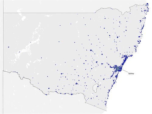
Figure 2. Maps showing SA1-level population and employment density in 2016 in the Sydney UCL.

Maps of the Sydney metropolitan area showing the rail and ferry routes, which are focused on the CBD, and shaded for the densities of population and employment, which are stronger around the CBD.

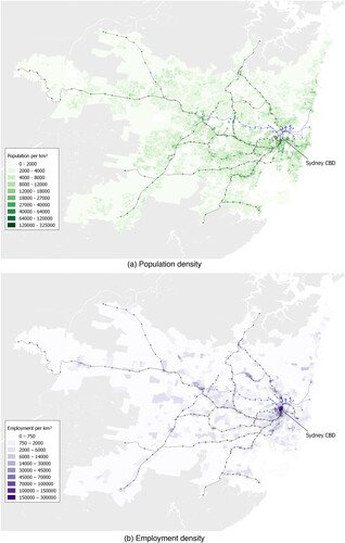
Figure 3. Maps showing SA1-level median residential property prices in the Sydney UCL in 2019 and 2021, both in 2019 dollars.

Maps of the Sydney metropolitan area shaded for the residential property price levels by SA1 in 2019 and 2021, which are generally higher near the CBD and beach but no patterns of differences between 2019 and 2021 are obvious.

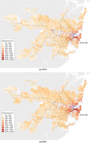
Table 1. Summary statistics for the main variables in the UCL-level dataset.

	Mean	Std. dev.	Minimum	Maximum
Data by UCL (532 observations):
Population in 2016	12,998	188,602	107	4,321,412
Distance to Sydney CBD (km)	311.1	187.8	0.0	933.4
Distance to coast (km)	107.2	132.2	0.1	610.5
Mean land elevation (m)	226.2	286.0	2.4	1,846.8
Mean January temperature (°C)	29.0	2.8	21.9	37.1
Mean July temperature (°C)	16.0	2.7	5.6	20.6
Mean annual rainfall (mm)	934.6	358.2	244.5	1884.8
Population in 2016 / population in 2011	1.052	0.068	0.915	1.492
Mean age	42.4	3.8	33.6	54.7
Proportion of adults with year-10 education	0.831	0.035	0.759	0.914
Proportion of adults with university degree	0.151	0.056	0.060	0.324
Rate of breaking and entering (per 100 k residents)	108.8	99.4	73.2	832.2
Rate of robbery (per 100 k residents)	6.5	0.5	6.4	12.5
Rate of non-domestic assault (per 100 k residents)	138.7	31.6	131.7	709.4
Data by UCL and year (5922 observations):
Number of non-strata residential property transactions	170.1	1826.5	1	50,665
Median size of property (m^2)	1004.3	522.8	200	4000
Median purchase price (AUD)	472,761.5	324,518.2	33,000	5,000,000
Median purchase price per m^2 (AUD)	550.4	468.2	100.1	8750.0

Table 2. Summary statistics for the main variables in the Sydney SA1-level dataset.

	Mean	Std. dev.	Minimum	Maximum
Data by SA1 (9870 observations):
Travel time by road to Sydney CBD (minutes)	28.1	13.3	0.4	77.3
Travel time by road to beach (minutes)	30.3	17.3	0.2	94.8
Travel time by road to Sydney Harbour (minutes)	24.3	13.8	0.1	77.2
Travel time by rail or ferry to Sydney CBD (minutes)	47.6	21.0	0.7	119.7
Mean land elevation (m)	55.9	46.9	0.6	460.6
Mean January temperature (°C)	27.8	1.2	25.2	30.5
Mean July temperature (°C)	17.2	0.3	15.8	17.8
Mean annual rainfall (mm)	965.1	165.3	301.9	1212.0
Population in 2016 / population in 2011	1.106	0.164	0.300	11.600
Mean age	37.3	2.7	31.0	51.9
Proportion of adults with year-10 education	0.875	0.051	0.667	1.000
Proportion of adults with university degree	0.322	0.140	0.000	0.623
Rate of breaking and entering (per 100 k residents)	252.8	276.2	73.2	832.2
Rate of robbery (per 100 k residents)	11.9	15.9	6.4	67.4
Rate of non-domestic assault (per 100 k residents)	235.1	249.0	131.7	1029.3
Data by SA1 and year (86,572 observations):
Number of non-strata residential property transactions	5.1	8.8	1	867
Median size of property (m^2)	590.4	263.4	100	4000
Median purchase price (AUD)	1,401,786.4	1,410,314.7	36,050	150,000,000
Median purchase price per m^2 (AUD)	2992.6	3380.3	201.3	83,891.8

Figure 4. Quarterly median property prices per square metre from 2016 to June 2023, normalised to the first quarter of 2020. The plots compare towns or cities in New South Wales by population and neighbourhoods in the Sydney metropolitan area by road travel time to the CBD.

Plots of quarterly property prices by town and city population and by distance of neighbourhood in the Sydney metropolitan area, normalised to the first quarter of 2020. No consistent patterns are evident before Q1 2020, but after that the prices grow in relative terms in medium-sized cities and in less central parts of Sydney.

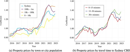
Table 3. OLS estimation results for the UCL-level relationships between (log) residential property prices by year and the (log) UCL population, distance to Sydney, and distance to the coast, with the populations and distances in separate regressions.

Year	(1) 2014	(2) 2015	(3) 2016	(4) 2017	(5) 2018	(6) 2019	(7) 2020	(8) 2021	(9) 2022
Panel A. Estimates using UCL population in 2016
ln (population)	0.135^a (0.015)	0.150^a (0.015)	0.158^a (0.014)	0.162^a (0.015)	0.161^a (0.014)	0.147^a (0.014)	0.148^a (0.015)	0.160^a (0.016)	0.153^a (0.017)
R^2	0.60	0.62	0.64	0.67	0.69	0.69	0.68	0.71	0.72
Panel B. Estimates using distance to Sydney CBD
ln (distance to Sydney CBD)	−0.163^a (0.045)	−0.208^a (0.052)	−0.204^a (0.057)	−0.217^a (0.057)	−0.212^a (0.056)	−0.167^a (0.046)	−0.167^a (0.047)	−0.183^a (0.049)	−0.181^a (0.052)
R^2	0.58	0.61	0.62	0.65	0.67	0.66	0.65	0.69	0.70
Panel C. Estimates using distance to nearest coast
ln (distance to coast)	−0.099^a (0.014)	−0.089^a (0.013)	−0.110^a (0.014)	−0.121^a (0.015)	−0.145^a (0.016)	−0.150^a (0.014)	−0.166^a (0.019)	−0.171^a (0.015)	−0.197^a (0.019)
R^2	0.65	0.66	0.67	0.70	0.71	0.71	0.71	0.73	0.74
Number of observations	483	492	498	497	493	490	497	499	506

Note: Robust standard errors in parentheses; a, b, c denote significance at 1%, 5%, 10%; the dependent variable in each regression is the (log) median sale price per square metre for residential properties in the UCL in the given year; all regressions include the full range of controls for geography, climate, demography and crime, the coefficients on which are not displayed.

Figure 5. Coefficients on (log) UCL population and distances to Sydney and the coast, from separate regressions.

The coefficients on proximity in the property-prices of towns and cities, estimated from separate regressions, show no clear pattern or effect of the pandemic.

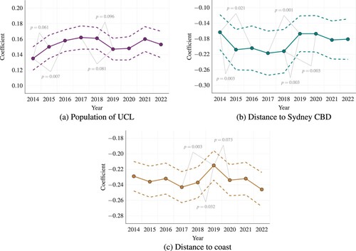
Figure 6. Coefficients on (log) UCL population and distances to Sydney and the coast, from the same regression for each year.

The coefficients on proximity in the property-prices of towns and cities, estimated from the same regressions, show no clear pattern or effect of the pandemic.

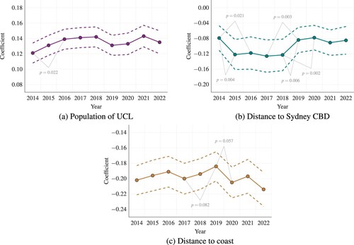
Table 4. OLS estimation results for the UCL-level relationships between (log) residential property prices by year and the (log) UCL population, distance to Sydney, and distance to the coast, with the populations and distances in the same regression for each year.

	(1)	(2)	(3)	(4)	(5)	(6)	(7)	(8)	(9)
Year	2014	2015	2016	2017	2018	2019	2020	2021	2022
ln (population)	0.121^a	0.131^a	0.139^a	0.141^a	0.142^a	0.131^a	0.133^a	0.143^a	0.135^a
	(0.013)	(0.013)	(0.013)	(0.013)	(0.013)	(0.013)	(0.014)	(0.014)	(0.015)
ln (distance to Sydney CBD)	−0.079^b	−0.122^a	−0.118^a	−0.118^a	−0.126^a	−0.084^b	−0.078^b	−0.091^a	−0.085^b
	(0.032)	(0.039)	(0.042)	(0.042)	(0.041)	(0.033)	(0.032)	(0.033)	(0.036)
ln (distance to coast)	−0.202^a	−0.196^a	−0.191^a	−0.200^a	−0.194^a	−0.184^a	−0.205^a	−0.197^a	−0.214^a
	(0.019)	(0.020)	(0.020)	(0.020)	(0.020)	(0.019)	(0.020)	(0.022)	(0.022)
R^2	0.71	0.74	0.74	0.77	0.78	0.76	0.76	0.78	0.79
Number of observations	483	492	498	497	493	490	497	499	506

Note: Robust standard errors in parentheses; a, b, c denote significance at 1%, 5%, 10%; the dependent variable in each regression is the (log) median sale price per square metre for residential properties in the UCL in the given year; all regressions include the full range of controls for geography, climate, demography and crime, the coefficients on which are not displayed.

Table 5. OLS estimation results for the UCL-level relationships between (log) residential property prices in 2019 and 2021 and the first two moments of (log) UCL population, distance to Sydney and distance to the coast.

	(1)	(2)	(3)	(4)	(5)	(6)	(7)	(8)
Year	2019	2021	2019	2021	2019	2021	2019	2021
ln (population)	0.228^a	0.286^a					0.350^a	0.450^a
	(0.079)	(0.091)					(0.089)	(0.093)
	[p = 0.199]						[p = 0.078]
ln (population)^2	-0.005	-0.008					−0.014^a	−0.020^a
	(0.005c)	(0.005)					(0.005)	(0.006)
	[p = 0.255]						[p = 0.088]
ln (distance to Sydney CBD)			−0.040^c	−0.052^b			−0.069^b	−0.104^a
			(0.021)	(0.025)			(0.027)	(0.028)
			[p = 0.096]				[p = 0.016]
ln (distance to Sydney CBD)^2			−0.020^a	−0.020^a			−0.006	−0.003
			(0.003)	(0.004)			(0.004)	(0.004)
			[p = 0.833]				[p = 0.237]
ln (distance to coast)					−0.147^a	−0.164^a	−0.168^a	−0.186^a
					(0.027)	(0.030)	(0.026)	(0.030)
					[p = 0.285]		[p = 0.272]
ln (distance to coast)^2					−0.031^a	−0.030^a	−0.004	−0.002
					(0.008)	(0.009)	(0.009)	(0.010)
					[p = 0.898]		[p = 0.676]
R^2	0.69	0.71	0.67	0.69	0.72	0.73	0.77	0.79
Number of observations	490	499	490	499	490	499	490	499

Note: Robust standard errors in parentheses and p-values or differences between coefficients in square brackets; a, b, c denote significance at 1%, 5%, 10%; the dependent variable in each regression is the (log) median sale price per square metre for residential properties in the UCL in the given year; all regressions include the full range of controls for geography, climate, demography and crime, the coefficients on which are not displayed.

Figure 7. Coefficients on (log) travel times by road to the Sydney CBD, the beach and Sydney Harbour and by rail or ferry to the CBD, from separate regressions.

The coefficients on proximity in the property-prices of Sydney SA1s, estimated from separate regressions, show (i) decreased premiums on proximity to the CBD by road or rail and ferry during the pandemic and (ii) a steady increase in the premium on proximity to the beach since 2015 that continues through the pandemic with no obvious change.

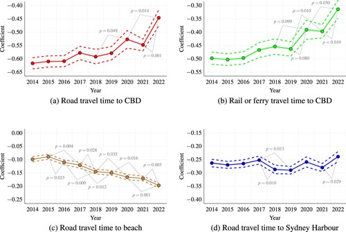
Table 6. OLS estimation results for the SA1-level relationships between (log) residential property prices by year in the Sydney metropolitan area and each type of (log) travel time, with the travel times in separate regressions.

Year	(1) 2014	(2) 2015	(3) 2016	(4) 2017	(5) 2018	(6) 2019	(7) 2020	(8) 2021	(9) 2022
Panel A. Estimates using travel time by road to Sydney CBD
ln (travel time by road to Sydney CBD)	−0.617^a (0.021)	−0.610^a (0.021)	−0.609^a (0.021)	−0.578^a (0.025)	−0.592^a (0.027)	−0.579^a (0.025)	−0.527^a (0.033)	−0.548^a (0.022)	−0.446^a (0.030)
R^2	0.78	0.78	0.78	0.78	0.77	0.77	0.75	0.79	0.76
Panel B. Estimates using travel time by rail or ferry to Sydney CBD
ln (travel time by rail / ferry to Sydney CBD)	−0.498^a (0.023)	−0.503^a (0.022)	−0.497^a (0.023)	−0.467^a (0.028)	−0.454^a (0.029)	−0.463^a (0.027)	−0.391^a (0.036)	−0.397^a (0.025)	−0.314^a (0.034)
R^2	0.77	0.77	0.77	0.77	0.75	0.75	0.74	0.78	0.76
Panel C. Estimates using travel time by road to nearest beach
ln (travel time by road to beach)	−0.099^a (0.010)	−0.089^a (0.009)	−0.110^a (0.009)	−0.121^a (0.011)	−0.145^a (0.009)	−0.150^a (0.009)	−0.166^a (0.010)	−0.171^a (0.009)	−0.197^a (0.009)
R^2	0.76	0.76	0.76	0.76	0.75	0.75	0.74	0.78	0.77
Panel D. Estimates using travel time by road to Sydney Harbour
ln (travel time by road to Sydney Harbour)	−0.263^a (0.014)	−0.270^a (0.013)	−0.265^a (0.014)	−0.252^a (0.015)	−0.287^a (0.016)	−0.290^a (0.014)	−0.259^a (0.019)	−0.280^a (0.015)	−0.239^a (0.019)
R^2	0.77	0.78	0.77	0.78	0.76	0.76	0.75	0.79	0.77
Number of observations	8041	7997	7841	7840	7570	7687	7763	8108	7988

Note: robust standard errors in parentheses; a, b, c denote significance at 1%, 5%, 10%; the dependent variable in each regression is the (log) median sale price per square metre for residential properties in the SA1 in the given year; all regressions include the full range of controls for geography, climate, demography, and crime, the coefficients on which are not displayed.

Figure 8. Coefficients on (log) travel times by road to the Sydney CBD, the beach and Sydney Harbour and by rail or ferry to the CBD, from the same regression for each year.

The coefficients on proximity in the property-prices of Sydney SA1s, estimated from the same regressions, show (i) a decreased premium on proximity to the CBD by rail or ferry in 2020 and 2021, (ii) a decreased premium on proximity to the CBD by road in 2022, and (iii) a steady increase in the premium on proximity to the beach since 2015 that continues through the pandemic with no obvious change.

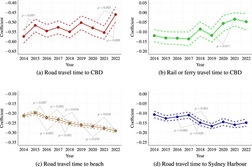
Table 7. OLS estimation results for the SA1-level relationships between (log) residential property prices by year in the Sydney metropolitan area and each type of (log) travel time, with all four types of travel time in the same regression for each year.

Year	(1) 2014	(2) 2015	(3) 2016	(4) 2017	(5) 2018	(6) 2019	(7) 2020	(8) 2021	(9) 2022
ln (travel time by road to Sydney CBD)	−0.573^a	−0.516^a	−0.545^a	−0.526^a	−0.549^a	−0.502^a	−0.529^a	−0.553^a	−0.460^a
	(0.034)	(0.033)	(0.033)	(0.033)	(0.032)	(0.035)	(0.039)	(0.034)	(0.038)
ln (travel time by rail / ferry to Sydney CBD)	−0.119^a	−0.131^a	−0.132^a	−0.136^a	−0.085^b	−0.118^a	−0.056	−0.034	−0.047
	(0.031)	(0.032)	(0.032)	(0.036)	(0.037)	(0.034)	(0.042)	(0.033)	(0.042)
ln (travel time by road to beach)	−0.212^a	−0.197^a	−0.222^a	−0.232^a	−0.251^a	−0.260^a	−0.267^a	−0.277^a	−0.290^a
	(0.009)	(0.009)	(0.008)	(0.011)	(0.009)	(0.009)	(0.010)	(0.009)	(0.009)
ln (travel time by road to Sydney) Harbour)	−0.106^a	−0.126^a	−0.118^a	−0.109^a	−0.148^a	−0.166^a	−0.144^a	−0.159^a	−0.148^a
	(0.017)	(0.014)	(0.015)	(0.016)	(0.015)	(0.013)	(0.018)	(0.015)	(0.019)
R^2	0.80	0.80	0.80	0.81	0.79	0.80	0.78	0.83	0.80
Number of observations	8041	7997	7841	7840	7570	7687	7763	8108	7988

Note: Robust standard errors in parentheses; a, b, c denote significance at 1%, 5%, 10%; the dependent variable in each regression is the (log) median sale price per square metre for residential properties in the SA1 in the given year; all regressions include the full range of controls for geography, climate, demography and crime, the coefficients on which are not displayed.

DATA AVAILABILITY STATEMENT

The data used in this research were assembled from several public sources, as detailed in the Data section above, and are free to download with no permission required. The primary sources were the New South Wales Valuer General and the Australian Bureau of Statistics. Other data were from the Open Source Routing Machine, Transport for NSW, Geoscience Australia, the Bureau of Meteorology, and the New South Wales Bureau of Crime Statistics and Research.