A simple immunosensor for thyroid stimulating hormone

Figures & data

Figure 1. (A) EIS spectra of each immobilisation step of the ANTI_TSH [-■-■-(pink): Au-BARE, -▲-▲- (green): Au-BARE-CYS, -●-●- (red): Au-BARE-CYS-PAMAM, -♦-♦- (blue): Au-BARE-CYS-PAMAM-ANTI_TSH]. (B) Cyclic voltammograms of each immobilisation step of the ANTI_TSH [-■-■-(blue): Au-BARE, -▲-▲- (light green): Au-BARE-CYS, -●-●- (red): Au-BARE-CYS-PAMAM, -♦-♦- (dark green): Au-BARE-CYS-PAMAM-ANTI_TSH].

Scheme 1. Construction of the biosensor.

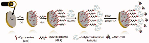
Figure 2. Calibration graphs of biosensors prepared using different cysteamine concentration; [-●-●-(blue): 10 mM CYS, -●-●- (dark grey): 50 mM CYS, -●-●- (green): 100 mM CYS, -●-●- (red): 150 mM CYS].

Figure 3. Calibration graphs of biosensors prepared using different cysteamine incubation times; [-●-●-(blue): 30 min, -●-●- (green): 60 min, -●-●- (orange): 90 min].

Figure 4. Calibration graphs of biosensors prepared using different concentrations of PAMAM (w/v); [-●-●-(blue): 1.0%, -●-●- (red): 1.5%, -●-●- (green): 2.0%].

Figure 5. Calibration graphs of biosensors fabricated using different ANTI-TSH concentrations [-●-●-(green): 1 ng/5 µL, -●-●- (red): 1 ng/5 µL, -●-●- (blue): 1 ng/5 µL].

Table 1. R² values and curve equations obtained from biosensors fabricated using different ANI-TSH concentrations.

Anti-TSH (ng/5µL)	R^2	y
1	0.9653	y = 0.6717x + 0.037
2.5	0.9897	y = 0.6386x + 0.0261
5	0.8252	y = 0.9625x + 0.0679

Figure 6. SEM images of the designed biosensor; Au-BARE (A), Au-BARE-CYS-PAMAM (B), Au-BARE-CYS-PAMAM-ANTI_TSH (C).

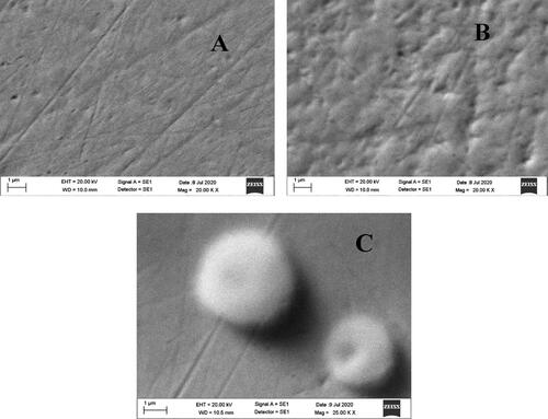
Figure 7. EDX elemental mapping and spectra of Au-BARE (A), Au-BARE-CYS (B), Au-BARE-CYS-PAMAM (C).

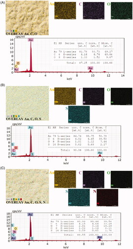
Figure 8. (A) Electrochemical impedance spectra obtained as Nyquist curves for different TSH concentrations. (B) Cyclic voltammograms obtained for different TSH concentrations.

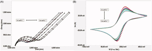
Figure 9. Calibration graph of proposed biosensor.

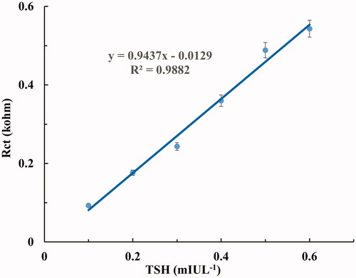
Table 2. Comparison between the proposed biosensor and other methods.

Method	Dynamic range (mIUL^−1)	LOD (mIUL^−1)	Ref.
Microfluidic electrochemical enzyme İmmunoassay	1–8	2.40	[33]
Lateral flow immunochromatographic assay with UV detection	0.31–5	0.31	[34]
Lab-on-a chip operated with enzyme immunoassay with chemiluminescence detection	1.9–55	1.90	[35]
Surface plasmon resonance based gold nanobiosensor	0.4–12.5	1.71	[36]
Kinetic exclusion analysis	0.05–100	0.4	[37]
Square-wave voltammograms based electrochemical immunosensor	0.2–20	0.04	[38]
Linear sweep voltammetry Electrochemical immunosensor	0.02–100	0.012	[39]
EIS based biosensor electrochemical İmmunosensor	0.001–150	0.001	[44]
Proposed biosensor	0.1–0.6	0.026

Table 3. Reproducibility of biosensor.

Biosensor number	R^2	Equation	Dynamic range (mIUL^−1)
1	0.9771	y = 1.142x + 0.0265	0.1–0.6
2	0.9821	y = 0.9858x − 0.0351	0.1–0.6
3	0.9615	y = 0.8519x − 0.0428	0.1–0.6
4	0.9814	y = 0.8933x + 0.0215	0.1–0.6
5	0.9882	y = 0.9437x − 0.0129	0.1–0.6
6	0.9748	y = 1.046x + 0.0371	0.1–0.6
7	0.9689	y = 0.9018x − 0.0346	0.1–0.6

Table 4. The analysis results of TSH in artificial serum samples.

TSH concentration of artificial serum (mIUL^−1)	Measured TSH concentration (mIUL^−1)	Recovery (%)
0.1	0.119	119.0
0.2	0.198	99.0
0.3	0.270	90.0
0.4	0.397	99.25
0.5	0.502	100.4
0.6	0.611	101.8

Shamsi MH, Choi K, Ng AH, et al. A digital microfluidic electrochemical immunoassay. Lab Chip. 2014;14(3):547–554.

 PubMed Web of Science ®Google Scholar

Langén VL, Niiranen TJ, Puukka P, et al. Thyroid-stimulating hormone and risk of sudden cardiac death, total mortality and cardiovascular morbidity. Clin Endocrinol. 2018;88(1):105–113.

 PubMed Web of Science ®Google Scholar

Jung W, Han J, Kai J, et al. An innovative sample-to-answer polymer lab-on-a-chip with on-chip reservoirs for the POCT of thyroid stimulating hormone (TSH). Lab Chip. 2013;13(23):4653–4662.

 PubMed Web of Science ®Google Scholar

Salahvarzi A, Mahani M, Torkzadeh-Mahani M, et al. Localized surface plasmon resonance based gold nanobiosensor: determination of thyroid stimulating hormone. Anal Biochem. 2017;516:1–5.

 PubMed Web of Science ®Google Scholar

Wani TA, Zargar S, Wakil SM, et al. New analytical application of antibody-based biosensor in estimation of thyroid-stimulating hormone in serum. Bioanalysis. 2016;8(7):625–632.

 PubMed Web of Science ®Google Scholar

Smaniotto A, Mezalira DZ, Zapp E, et al. Electrochemical immunosensor based on an azo compound for thyroid-stimulating hormone detection. Microchem J. 2017;133:510–517.

 Web of Science ®Google Scholar

Wang H, Wu X, Dong P, et al. Electrochemical biosensor based on ınterdigitated electrodes for determination of thyroid stimulating hormone. Int J Electrochem Sci. 2014;9(1):12.

 Web of Science ®Google Scholar

Saxena R, Srivastava S. A sensitive and one-step quantification of thyroid stimulating hormone using nanobiosensor. Mater Today: Proc. 2019;18(3):1351–1357.

 Google Scholar